| size(Map<K.V>) |
Returns the number of elements in the map type. |
| size(Array<T>) |
Returns the number of elements in the array type. |
| map_keys(Map<K.V>) |
Returns an unordered array containing the keys of the input map. |
| map_values(Map<K.V>) |
Returns an unordered array containing the values of the input map. |
| array_contains(Array<T>, value) |
Returns TRUE if the array contains value. |
| sort_array(Array<T>) |
Sorts the input array in ascending order according to the natural ordering of the array elements and returns it |
| binary(string or binary) |
Casts the parameter into a binary. |
| cast(expr as ‘type’) |
Converts the results of the expression expr to the given type. |
| from_unixtime(bigint unixtime[, string format]) |
Converts the number of seconds from unix epoch (1970-01-01 00:00:00 UTC) to a string. |
| unix_timestamp() |
Gets current Unix timestamp in seconds. |
| unix_timestamp(string date) |
Converts time string in format yyyy-MM-dd HH:mm:ss to Unix timestamp (in seconds). |
| to_date(string timestamp) |
Returns the date part of a timestamp string. |
| year(string date) |
Returns the year part of a date. |
| quarter(date/timestamp/string) |
Returns the quarter of the year for a date. |
| month(string date) |
Returns the month part of a date or a timestamp string. |
| day(string date) dayofmonth(date) |
Returns the day part of a date or a timestamp string. |
| hour(string date) |
Returns the hour of the timestamp. |
| minute(string date) |
Returns the minute of the timestamp. |
| second(string date) |
Returns the second of the timestamp. |
| weekofyear(string date) |
Returns the week number of a timestamp string. |
| extract(field FROM source) |
Retrieve fields such as days or hours from source.
Source must be a date, timestamp, interval or a string that can be converted into either a date or timestamp. |
| datediff(string enddate, string startdate) |
Returns the number of days from startdate to enddate. |
| date_add(date/timestamp/string startdate, tinyint/smallint/int days) |
Adds a number of days to startdate. |
| date_sub(date/timestamp/string startdate, tinyint/smallint/int days) |
Subtracts a number of days to startdate. |
| from_utc_timestamp({any primitive type} ts, string timezone) |
Converts a timestamp in UTC to a given timezone. |
| to_utc_timestamp({any primitive type} ts, string timezone) |
Converts a timestamp in a given timezone to UTC. |
| current_date |
Returns the current date. |
| current_timestamp |
Returns the current timestamp. |
| add_months(string start_date, int num_months, output_date_format) |
Returns the date that is num_months after start_date. |
| last_day(string date) |
Returns the last day of the month which the date belongs to. |
| next_day(string start_date, string day_of_week) |
Returns the first date which is later than start_date and named as day_of_week. |
| trunc(string date, string format) |
Returns date truncated to the unit specified by the format. |
| months_between(date1, date2) |
Returns number of months between dates date1 and date2. |
| date_format(date/timestamp/string ts, string fmt) |
Converts a date/timestamp/string to a value of string in the format specified by the date format fmt. |
| if(boolean testCondition, T valueTrue, T valueFalseOrNull) |
Returns valueTrue when testCondition is true, returns valueFalseOrNull otherwise. |
| isnull( a ) |
Returns true if a is NULL and false otherwise. |
| isnotnull ( a ) |
Returns true if a is not NULL and false otherwise. |
| nvl(T value, T default_value) |
Returns default value if value is null else returns value. |
| COALESCE(T v1, T v2, …) |
Returns the first v that is not NULL, or NULL if all v’s are NULL. |
| CASE a WHEN b THEN c [WHEN d THEN e]* [ELSE f] END |
When a = b, returns c; when a = d, returns e; else returns f. |
| nullif( a, b ) |
Returns NULL if a=b; otherwise returns a. |
| assert_true(boolean condition) |
Throw an exception if ‘condition’ is not true, otherwise return null. |
| ascii(string str) |
Returns the numeric value of the first character of str. |
| base64(binary bin) |
Converts the argument from binary to a base 64 string. |
| character_length(string str) |
Returns the number of UTF-8 characters contained in str. |
| chr(bigint |
double A) |
| concat(string |
binary A, string |
| context_ngrams(array<array<string>>, array<string>, int K, int pf) |
Returns the top-k contextual N-grams from a set of tokenized sentences. |
| concat_ws(string SEP, string A, string B…) |
Like concat() above, but with custom separator SEP. |
| decode(binary bin, string charset) |
Decodes the first argument into a String using the provided character set (one of ‘US-ASCII’, ‘ISO-8859-1’, ‘UTF-8’, ‘UTF-16BE’, ‘UTF-16LE’, ‘UTF-16’).
If either argument is null, the result will also be null. |
| elt(N int,str1 string,str2 string,str3 string,…) |
Return string at index number, elt(2,‘hello’,‘world’) returns ‘world’. |
| encode(string src, string charset) |
Encodes the first argument into a BINARY using the provided character set (one of ‘US-ASCII’, ‘ISO-8859-1’, ‘UTF-8’, ‘UTF-16BE’, ‘UTF-16LE’, ‘UTF-16’). |
| field(val T,val1 T,val2 T,val3 T,…) |
Returns the index of val in the val1,val2,val3,… list or 0 if not found. |
| find_in_set(string str, string strList) |
Returns the first occurance of str in strList where strList is a comma-delimited string. |
| format_number(number x, int d) |
Formats the number X to a format like '#,###,###.##', rounded to D decimal places, and returns the result as a string.
If D is 0, the result has no decimal point or fractional part. |
| get_json_object(string json_string, string path) |
Extracts json object from a json string based on json path specified, and returns json string of the extracted json object. |
| in_file(string str, string filename) |
Returns true if the string str appears as an entire line in filename. |
| instr(string str, string substr) |
Returns the position of the first occurrence of substr in str. |
| length(string A) |
Returns the length of the string. |
| locate(string substr, string str[, int pos]) |
Returns the position of the first occurrence of substr in str after position pos. |
| lower(string A) lcase(string A) |
Returns the string resulting from converting all characters of B to lower case. |
| lpad(string str, int len, string pad) |
Returns str, left-padded with pad to a length of len.
If str is longer than len, the return value is shortened to len characters. |
| ltrim(string A) |
Returns the string resulting from trimming spaces from the beginning(left hand side) of A. |
| ngrams(array<array<string>>, int N, int K, int pf) |
Returns the top-k N-grams from a set of tokenized sentences, such as those returned by the sentences() UDAF. |
| octet_length(string str) |
Returns the number of octets required to hold the string str in UTF-8 encoding. |
| parse_url(string urlString, string partToExtract [, string keyToExtract]) |
Returns the specified part from the URL.
Valid values for partToExtract include HOST, PATH, QUERY, REF, PROTOCOL, AUTHORITY, FILE, and USERINFO. |
| printf(String format, Obj… args) |
Returns the input formatted according do printf-style format strings. |
| regexp_extract(string subject, string pattern, int index) |
Returns the string extracted using the pattern. |
| regexp_replace(string INITIAL_STRING, string PATTERN, string REPLACEMENT) |
Returns the string resulting from replacing all substrings in INITIAL_STRING that match the java regular expression syntax defined in PATTERN with instances of REPLACEMENT. |
| repeat(string str, int n) |
Repeats str n times. |
| replace(string A, string OLD, string NEW) |
Returns the string A with all non-overlapping occurrences of OLD replaced with NEW. |
| reverse(string A) |
Returns the reversed string. |
| rpad(string str, int len, string pad) |
Returns str, right-padded with pad to a length of len. |
| rtrim(string A) |
Returns the string resulting from trimming spaces from the end(right hand side) of A. |
| sentences(string str, string lang, string locale) |
Tokenizes a string of natural language text into words and sentences, where each sentence is broken at the appropriate sentence boundary and returned as an array of words. |
| space(int n) |
Returns a string of n spaces. |
| split(string str, string pat) |
Splits str around pat (pat is a regular expression). |
| str_to_map(text[, delimiter1, delimiter2]) |
Splits text into key-value pairs using two delimiters.
Delimiter1 separates text into K-V pairs, and Delimiter2 splits each K-V pair.
Default delimiters are ‘,’ for delimiter1 and ‘:’ for delimiter2. |
| substr(string |
binary A, int start) |
| substring_index(string A, string delim, int count) |
Returns the substring from string A before count occurrences of the delimiter delim. |
| translate(string |
char |
| trim(string A) |
Returns the string resulting from trimming spaces from both ends of A. |
| unbase64(string str) |
Converts the argument from a base 64 string to BINARY. |
| upper(string A) ucase(string A) |
Returns the string resulting from converting all characters of A to upper case.
For example, upper(‘fOoBaR’) results in ‘FOOBAR’. |
| initcap(string A) |
Returns string, with the first letter of each word in uppercase, all other letters in lowercase.
Words are delimited by whitespace. |
| levenshtein(string A, string B) |
Returns the Levenshtein distance between two strings. |
| soundex(string A) |
Returns soundex code of the string. |
| mask(string str[, string upper[, string lower[, string number]]]) |
Returns a masked version of str. |
| mask_first_n(string str[, int n]) |
Returns a masked version of str with the first n values masked.
mask_first_n(“1234-5678-8765-4321”, 4) results in nnnn-5678-8765-4321. |
| mask_last_n(string str[, int n]) |
Returns a masked version of str with the last n values masked. |
| mask_show_first_n(string str[, int n]) |
Returns a masked version of str, showing the first n characters unmasked. |
| mask_show_last_n(string str[, int n]) |
Returns a masked version of str, showing the last n characters unmasked. |
| mask_hash(string |
char |
| java_method(class, method[, arg1[, arg2..]]) |
Synonym for reflect. |
| reflect(class, method[, arg1[, arg2..]]) |
Calls a Java method by matching the argument signature, using reflection. |
| hash(a1[, a2…]) |
Returns a hash value of the arguments. |
| current_user() |
Returns current user name from the configured authenticator manager. |
| logged_in_user() |
Returns current user name from the session state. |
| current_database() |
Returns current database name. |
| md5(string/binary) |
Calculates an MD5 128-bit checksum for the string or binary. |
| sha1(string/binary)sha(string/binary) |
Calculates the SHA-1 digest for string or binary and returns the value as a hex string. |
| crc32(string/binary) |
Computes a cyclic redundancy check value for string or binary argument and returns bigint value. |
| sha2(string/binary, int) |
Calculates the SHA-2 family of hash functions (SHA-224, SHA-256, SHA-384, and SHA-512). |
| aes_encrypt(input string/binary, key string/binary) |
Encrypt input using AES. |
| aes_decrypt(input binary, key string/binary) |
Decrypt input using AES. |
| version() |
Returns the Hive version. |
| count(expr) |
Returns the total number of retrieved rows. |
| sum(col), sum(DISTINCT col) |
Returns the sum of the elements in the group or the sum of the distinct values of the column in the group. |
| avg(col), avg(DISTINCT col) |
Returns the average of the elements in the group or the average of the distinct values of the column in the group. |
| min(col) |
Returns the minimum of the column in the group. |
| max(col) |
Returns the maximum value of the column in the group. |
| variance(col), var_pop(col) |
Returns the variance of a numeric column in the group. |
| var_samp(col) |
Returns the unbiased sample variance of a numeric column in the group. |
| stddev_pop(col) |
Returns the standard deviation of a numeric column in the group. |
| stddev_samp(col) |
Returns the unbiased sample standard deviation of a numeric column in the group. |
| covar_pop(col1, col2) |
Returns the population covariance of a pair of numeric columns in the group. |
| covar_samp(col1, col2) |
Returns the sample covariance of a pair of a numeric columns in the group. |
| corr(col1, col2) |
Returns the Pearson coefficient of correlation of a pair of a numeric columns in the group. |
| percentile(BIGINT col, p) |
Returns the exact pth percentile of a column in the group (does not work with floating point types).
p must be between 0 and 1. |
| percentile(BIGINT col, array(p1 [, p2]…)) |
Returns the exact percentiles p1, p2, … of a column in the group.
pi must be between 0 and 1. |
| percentile_approx(DOUBLE col, p [, B]) |
Returns an approximate pth percentile of a numeric column (including floating point types) in the group.
The B parameter controls approximation accuracy at the cost of memory.
Higher values yield better approximations, and the default is 10,000.
When the number of distinct values in col is smaller than B, this gives an exact percentile value. |
| percentile_approx(DOUBLE col, array(p1 [, p2]…) [, B]) |
Same as above, but accepts and returns an array of percentile values instead of a single one. |
| regr_avgx(independent, dependent) |
Equivalent to avg(dependent). |
| regr_avgy(independent, dependent) |
Equivalent to avg(independent). |
| regr_count(independent, dependent) |
Returns the number of non-null pairs used to fit the linear regression line. |
| regr_intercept(independent, dependent) |
Returns the y-intercept of the linear regression line, i.e. the value of b in the equation dependent = a * independent + b. |
| regr_r2(independent, dependent) |
Returns the coefficient of determination for the regression. |
| regr_slope(independent, dependent) |
Returns the slope of the linear regression line, i.e. the value of a in the equation dependent = a * independent + b. |
| regr_sxx(independent, dependent) |
Equivalent to regr_count(independent, dependent) * var_pop(dependent). |
| regr_sxy(independent, dependent) |
Equivalent to regr_count(independent, dependent) * covar_pop(independent, dependent). |
| regr_syy(independent, dependent) |
Equivalent to regr_count(independent, dependent) * var_pop(independent). |
| histogram_numeric(col, b) |
Computes a histogram of a numeric column in the group using b non-uniformly spaced bins.
The output is an array of size b of double-valued (x,y) coordinates that represent the bin centers and heights |
| collect_set(col) |
Returns a set of objects with duplicate elements eliminated. |
| collect_list(col) |
Returns a list of objects with duplicates. |
| ntile(INTEGER x) |
Divides an ordered partition into x groups called buckets and assigns a bucket number to each row in the partition.
This allows easy calculation of tertiles, quartiles, deciles, percentiles and other common summary statistics. |
| explode(ARRAY<T> a) |
Explodes an array to multiple rows.
Returns a row-set with a single column (col), one row for each element from the array. |
| explode(MAP<Tkey,Tvalue> m) |
Explodes a map to multiple rows.
Returns a row-set with a two columns (key,value) , one row for each key-value pair from the input map. |
| posexplode(ARRAY<T> a) |
Explodes an array to multiple rows with additional positional column of int type (position of items in the original array, starting with 0).
Returns a row-set with two columns (pos,val), one row for each element from the array. |
| inline(ARRAY<STRUCT<f1:T1,…,fn:Tn>> a) |
Explodes an array of structs to multiple rows.
Returns a row-set with N columns (N = number of top level elements in the struct), one row per struct from the array. |
| stack(int r,T1 V1,…,Tn/r Vn) |
Breaks up n values V1,…,Vn into r rows.
Each row will have n/r columns.
r must be constant. |
| json_tuple(string jsonStr,string k1,…,string kn) |
Takes JSON string and a set of n keys, and returns a tuple of n values. |
| parse_url_tuple(string urlStr,string p1,…,string pn) |
Takes URL string and a set of n URL parts, and returns a tuple of n values. |
 FIGURE 1.1: World’s capacity to store information
With the ambition to provide tools capable of searching all of this new digital information, many companies attempted to provide such functionality with what we know today as search engines, used when searching the web.
Given the vast amount of digital information, managing information at this scale was a challenging problem.
Search engines were unable to store all of the web page information required to support web searches in a single computer.
This meant that they had to split information into several files and store them across many machines.
This approach became known as the Google File System, and was presented in a research paper published in 2003 by Google.4
FIGURE 1.1: World’s capacity to store information
With the ambition to provide tools capable of searching all of this new digital information, many companies attempted to provide such functionality with what we know today as search engines, used when searching the web.
Given the vast amount of digital information, managing information at this scale was a challenging problem.
Search engines were unable to store all of the web page information required to support web searches in a single computer.
This meant that they had to split information into several files and store them across many machines.
This approach became known as the Google File System, and was presented in a research paper published in 2003 by Google.4
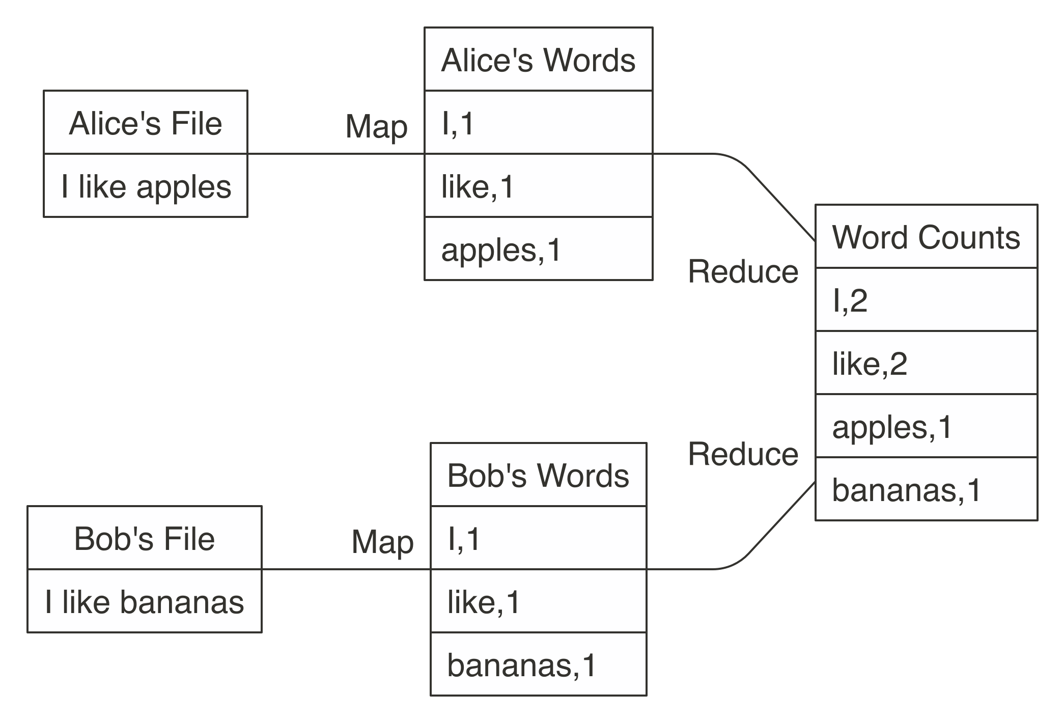 FIGURE 1.2: MapReduce example counting words across files
Counting words is often the most basic MapReduce example, but we can also use MapReduce for much more sophisticated and interesting applications.
For instance, we can use it to rank web pages in Google’s PageRank algorithm, which assigns ranks to web pages based on the count of hyperlinks linking to a web page and the rank of the page linking to it.
After these papers were released by Google, a team at Yahoo worked on implementing the Google File System and MapReduce as a single open source project.
This project was released in 2006 as Hadoop, with the Google File System implemented as the Hadoop Distributed File System (HDFS).
The Hadoop project made distributed file-based computing accessible to a wider range of users and organizations, making MapReduce useful beyond web data processing.
Although Hadoop provided support to perform MapReduce operations over a distributed file system, it still required MapReduce operations to be written with code every time a data analysis was run.
To improve upon this tedious process, the Hive project, released in 2008 by Facebook, brought Structured Query Language (SQL) support to Hadoop.
This meant that data analysis could now be performed at large scale without the need to write code for each MapReduce operation; instead, one could write generic data analysis statements in SQL, which are much easier to understand and write.
FIGURE 1.2: MapReduce example counting words across files
Counting words is often the most basic MapReduce example, but we can also use MapReduce for much more sophisticated and interesting applications.
For instance, we can use it to rank web pages in Google’s PageRank algorithm, which assigns ranks to web pages based on the count of hyperlinks linking to a web page and the rank of the page linking to it.
After these papers were released by Google, a team at Yahoo worked on implementing the Google File System and MapReduce as a single open source project.
This project was released in 2006 as Hadoop, with the Google File System implemented as the Hadoop Distributed File System (HDFS).
The Hadoop project made distributed file-based computing accessible to a wider range of users and organizations, making MapReduce useful beyond web data processing.
Although Hadoop provided support to perform MapReduce operations over a distributed file system, it still required MapReduce operations to be written with code every time a data analysis was run.
To improve upon this tedious process, the Hive project, released in 2008 by Facebook, brought Structured Query Language (SQL) support to Hadoop.
This meant that data analysis could now be performed at large scale without the need to write code for each MapReduce operation; instead, one could write generic data analysis statements in SQL, which are much easier to understand and write.
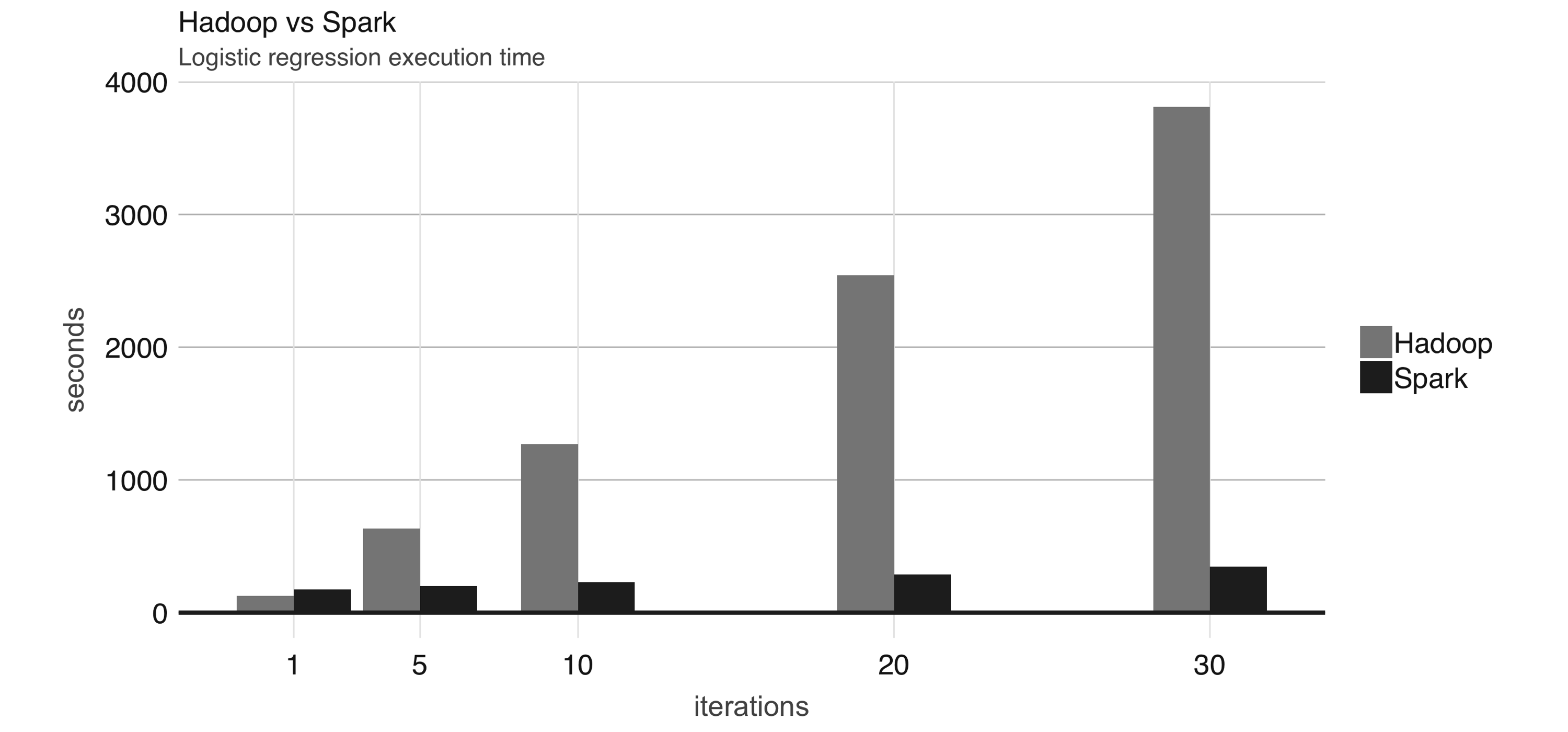 FIGURE 1.3: Logistic regression performance in Hadoop and Spark
Even though Spark is well known for its in-memory performance, it was designed to be a general execution engine that works both in-memory and on-disk.
For instance, Spark has set sorting7, for which data was not loaded in-memory; rather, Spark made improvements in network serialization, network shuffling, and efficient use of the CPU’s cache to dramatically enhance performance.
If you needed to sort large amounts of data, there was no other system in the world faster than Spark.
To give you a sense of how much faster and efficient Spark is, it takes 72 minutes and 2,100 computers to sort 100 terabytes of data using Hadoop, but only 23 minutes and 206 computers using Spark.
In addition, Spark holds the cloud sorting record, which makes it the most cost-effective solution for sorting large-datasets in the cloud.
FIGURE 1.3: Logistic regression performance in Hadoop and Spark
Even though Spark is well known for its in-memory performance, it was designed to be a general execution engine that works both in-memory and on-disk.
For instance, Spark has set sorting7, for which data was not loaded in-memory; rather, Spark made improvements in network serialization, network shuffling, and efficient use of the CPU’s cache to dramatically enhance performance.
If you needed to sort large amounts of data, there was no other system in the world faster than Spark.
To give you a sense of how much faster and efficient Spark is, it takes 72 minutes and 2,100 computers to sort 100 terabytes of data using Hadoop, but only 23 minutes and 206 computers using Spark.
In addition, Spark holds the cloud sorting record, which makes it the most cost-effective solution for sorting large-datasets in the cloud.
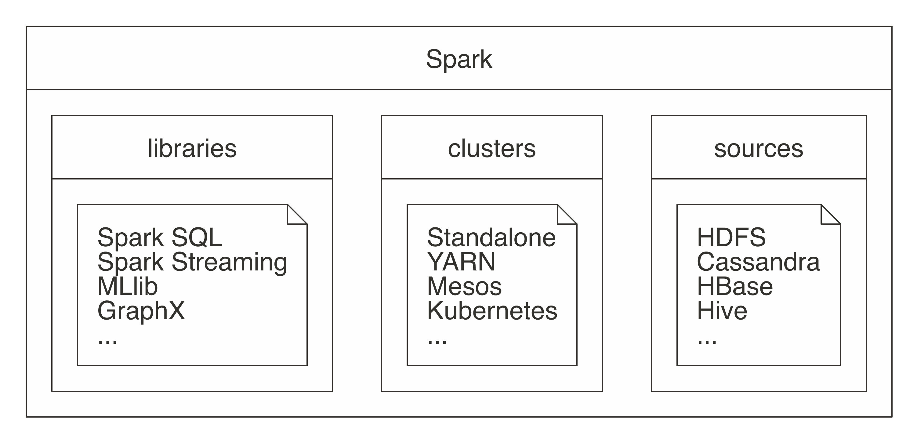 FIGURE 1.4: Spark as a unified analytics engine for large-scale data processing
Describing Spark as large scale implies that a good use case for Spark is tackling problems that can be solved with multiple machines.
For instance, when data does not fit on a single disk drive or into memory, Spark is a good candidate to consider.
However, you can also consider it for problems that might not be large scale, but for which using multiple computers could speed up computation.
For instance, CPU-intensive models and scientific simulations also benefit from running in Spark.
Therefore, Spark is good at tackling large-scale data-processing problems, usually known as big data (datasets that are more voluminous and complex than traditional ones) but it is also good at tackling large-scale computation problems, known as big compute (tools and approaches using a large amount of CPU and memory resources in a coordinated way).
Big data often requires big compute, but big compute does not necessarily require big data.
Big data and big compute problems are usually easy to spot—if the data does not fit into a single machine, you might have a big data problem; if the data fits into a single machine but processing it takes days, weeks, or even months to compute, you might have a big compute problem.
However, there is also a third problem space for which neither data nor compute is necessarily large scale and yet there are significant benefits to using cluster computing frameworks like Spark.
For this third problem space, there are a few use cases:
FIGURE 1.4: Spark as a unified analytics engine for large-scale data processing
Describing Spark as large scale implies that a good use case for Spark is tackling problems that can be solved with multiple machines.
For instance, when data does not fit on a single disk drive or into memory, Spark is a good candidate to consider.
However, you can also consider it for problems that might not be large scale, but for which using multiple computers could speed up computation.
For instance, CPU-intensive models and scientific simulations also benefit from running in Spark.
Therefore, Spark is good at tackling large-scale data-processing problems, usually known as big data (datasets that are more voluminous and complex than traditional ones) but it is also good at tackling large-scale computation problems, known as big compute (tools and approaches using a large amount of CPU and memory resources in a coordinated way).
Big data often requires big compute, but big compute does not necessarily require big data.
Big data and big compute problems are usually easy to spot—if the data does not fit into a single machine, you might have a big data problem; if the data fits into a single machine but processing it takes days, weeks, or even months to compute, you might have a big compute problem.
However, there is also a third problem space for which neither data nor compute is necessarily large scale and yet there are significant benefits to using cluster computing frameworks like Spark.
For this third problem space, there are a few use cases:
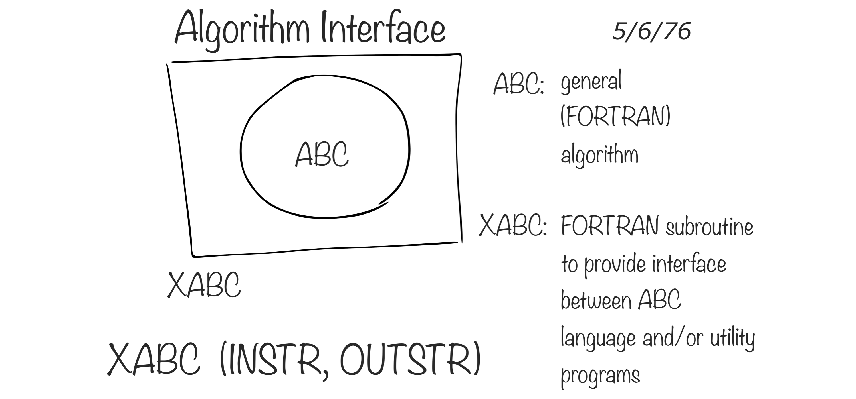 FIGURE 1.5: Interface language diagram by John Chambers (Rick Becker useR 2016)
R is a modern and free implementation of S.
Specifically, according to the R Project for Statistical Computing:
FIGURE 1.5: Interface language diagram by John Chambers (Rick Becker useR 2016)
R is a modern and free implementation of S.
Specifically, according to the R Project for Statistical Computing:
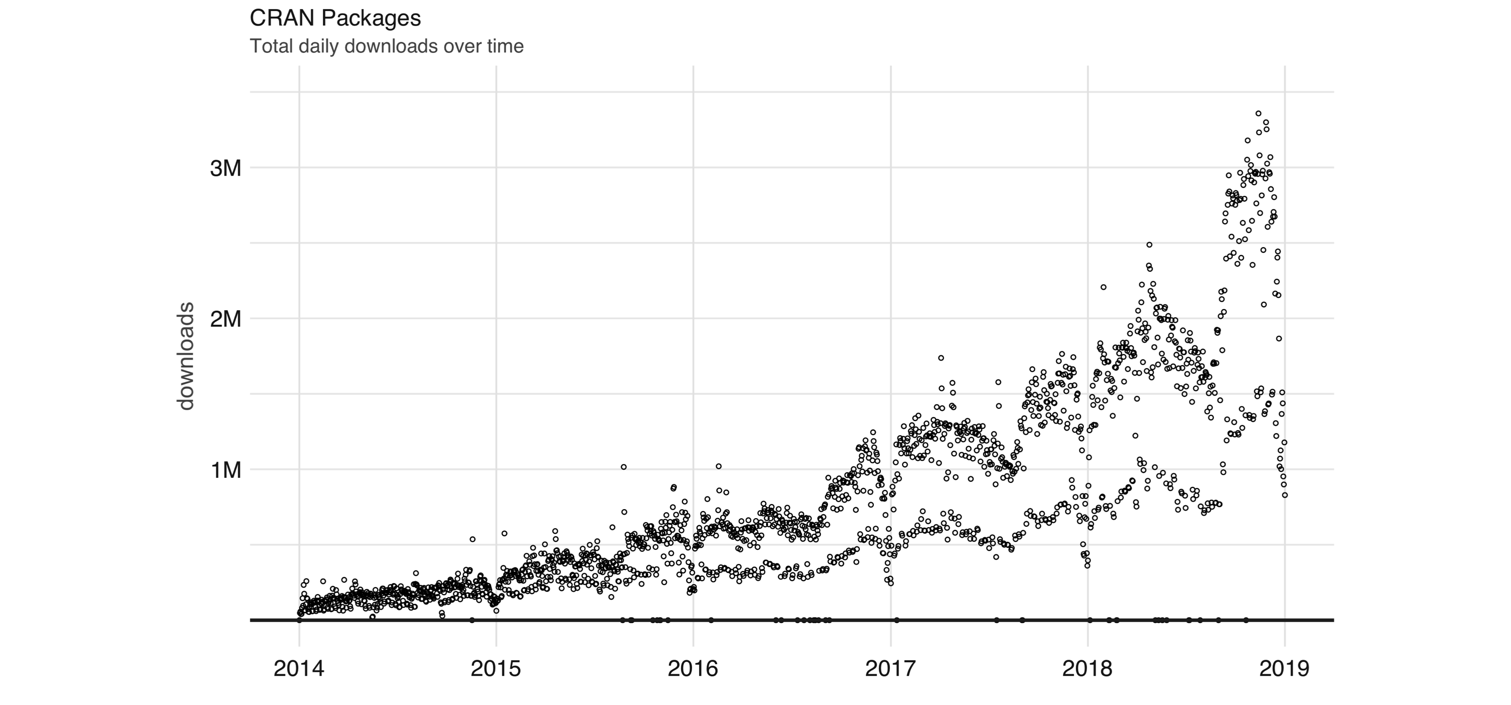 FIGURE 1.6: Daily downloads of CRAN packages
Aside from statistics, R is also used in many other fields.
The following areas are particularly relevant to this book:
FIGURE 1.6: Daily downloads of CRAN packages
Aside from statistics, R is also used in many other fields.
The following areas are particularly relevant to this book:
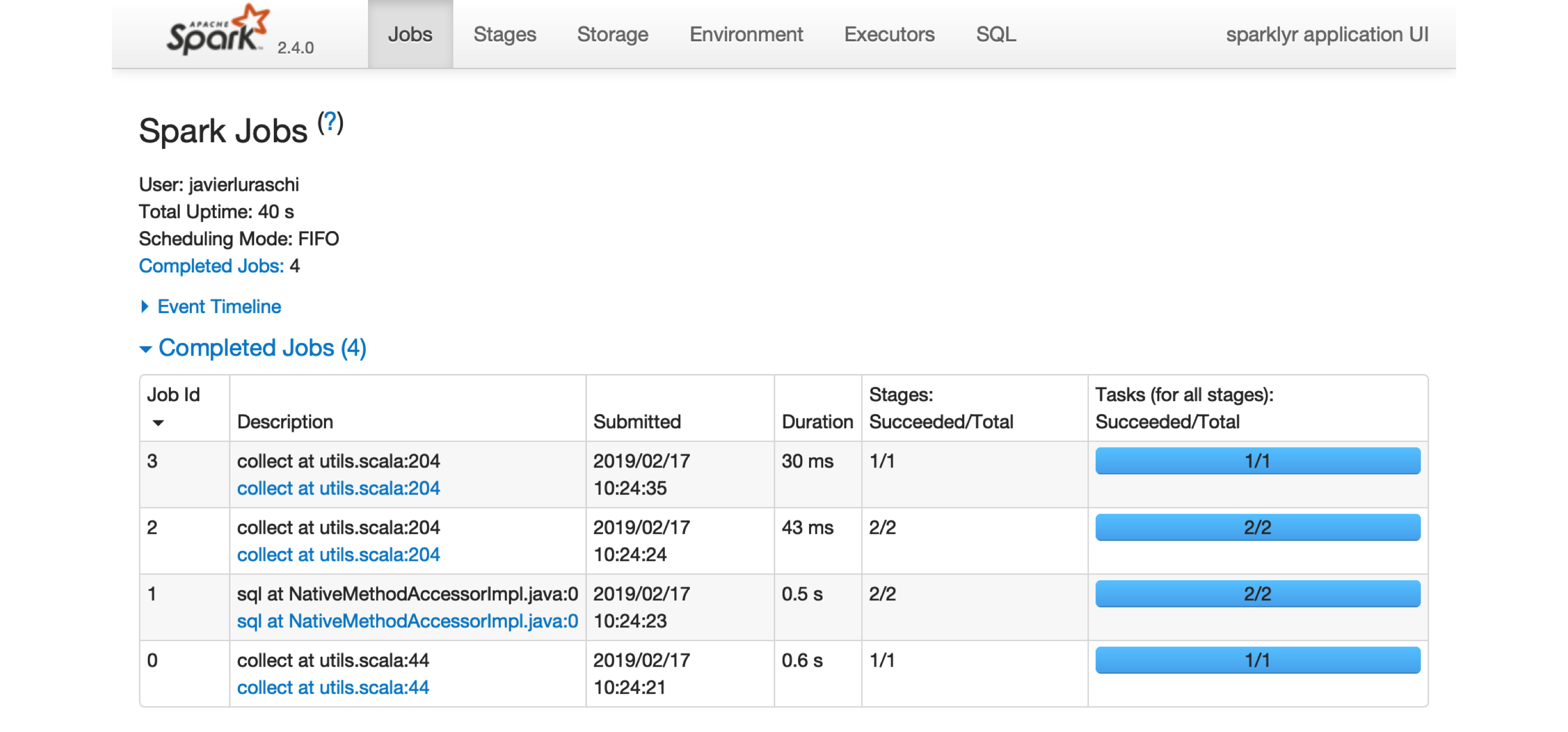 FIGURE 2.1: The Apache Spark web interface
Printing the
FIGURE 2.1: The Apache Spark web interface
Printing the 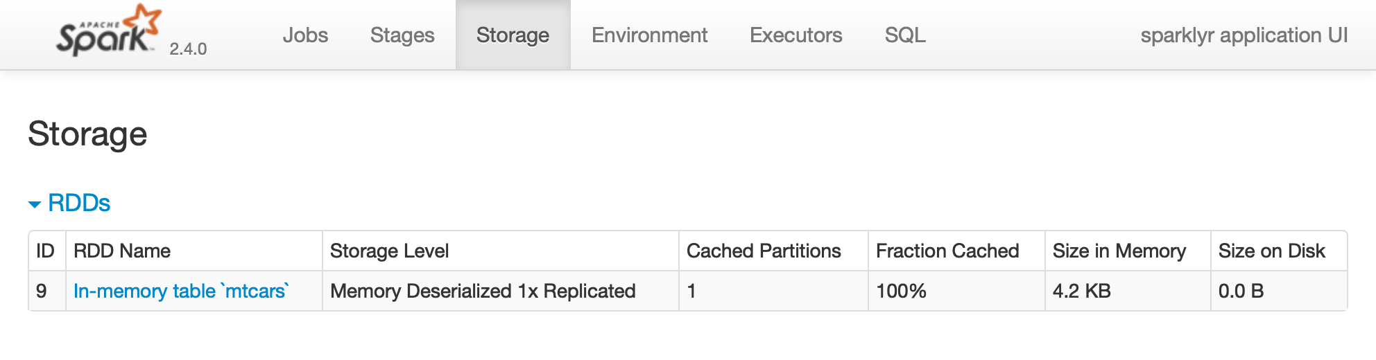 FIGURE 2.2: The Storage tab on the Apache Spark web interface
Notice that this dataset is fully loaded into memory, as indicated by the Fraction Cached column, which shows 100%; thus, you can see exactly how much memory this dataset is using through the Size in Memory column.
The Executors tab, shown in Figure 2.3, provides a view of your cluster resources.
For local connections, you will find only one executor active with only 2 GB of memory allocated to Spark, and 384 MB available for computation.
In Chapter 9 you will learn how to request more compute instances and resources, and how memory is allocated.
FIGURE 2.2: The Storage tab on the Apache Spark web interface
Notice that this dataset is fully loaded into memory, as indicated by the Fraction Cached column, which shows 100%; thus, you can see exactly how much memory this dataset is using through the Size in Memory column.
The Executors tab, shown in Figure 2.3, provides a view of your cluster resources.
For local connections, you will find only one executor active with only 2 GB of memory allocated to Spark, and 384 MB available for computation.
In Chapter 9 you will learn how to request more compute instances and resources, and how memory is allocated.
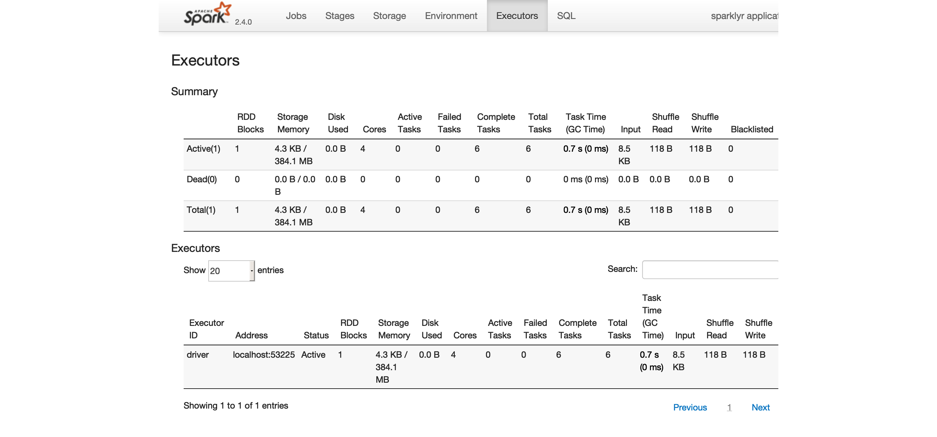 FIGURE 2.3: The Executors tab on the Apache Spark web interface
The last tab to explore is the Environment tab, shown in Figure 2.4; this tab lists all of the settings for this Spark application, which we look at in Chapter 9.
As you will learn, most settings don’t need to be configured explicitly, but to properly run them at scale, you need to become familiar with some of them, eventually.
FIGURE 2.3: The Executors tab on the Apache Spark web interface
The last tab to explore is the Environment tab, shown in Figure 2.4; this tab lists all of the settings for this Spark application, which we look at in Chapter 9.
As you will learn, most settings don’t need to be configured explicitly, but to properly run them at scale, you need to become familiar with some of them, eventually.
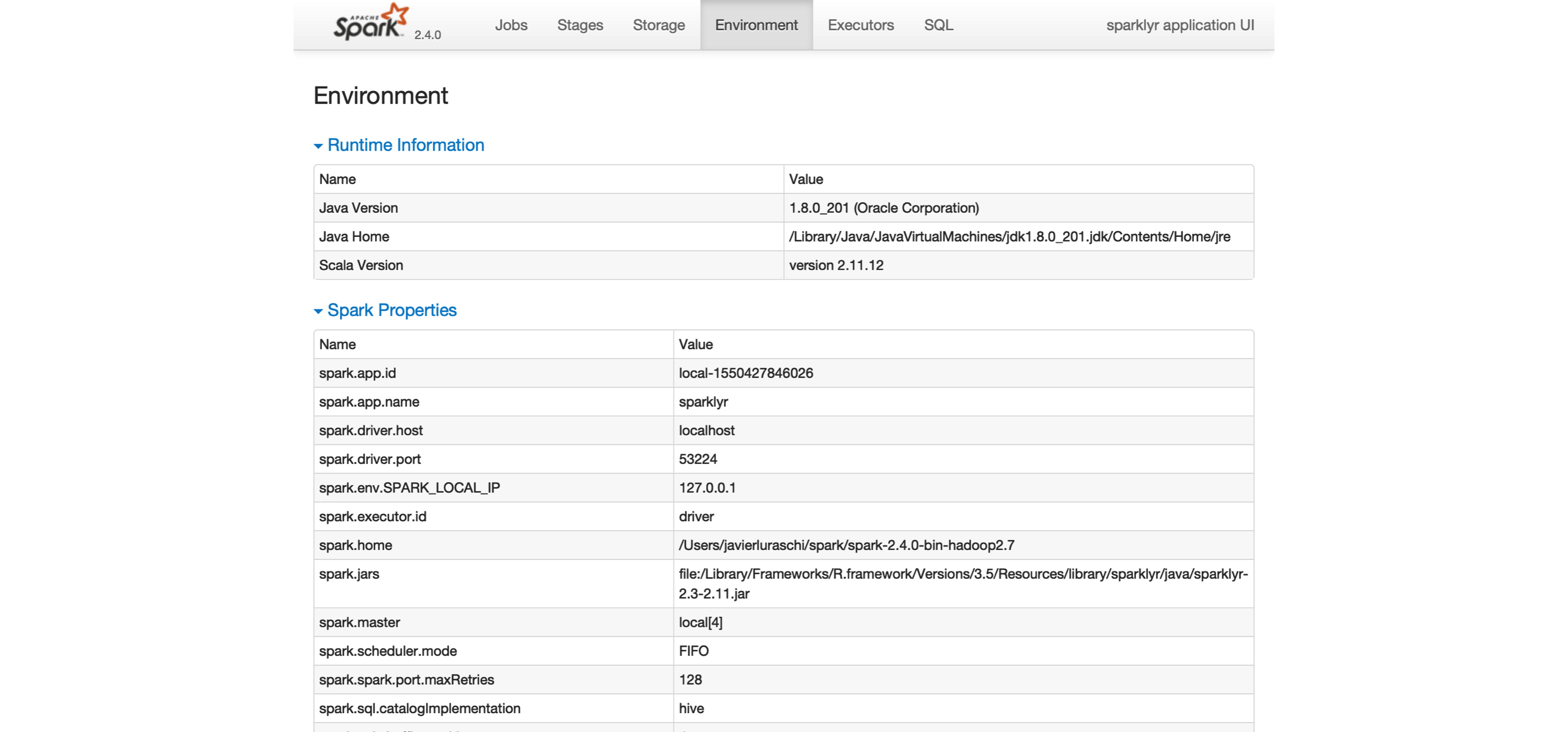 FIGURE 2.4: The Environment tab on the Apache Spark web interface
Next, you will make use of a small subset of the practices that we cover in depth in Chapter 3.
FIGURE 2.4: The Environment tab on the Apache Spark web interface
Next, you will make use of a small subset of the practices that we cover in depth in Chapter 3.
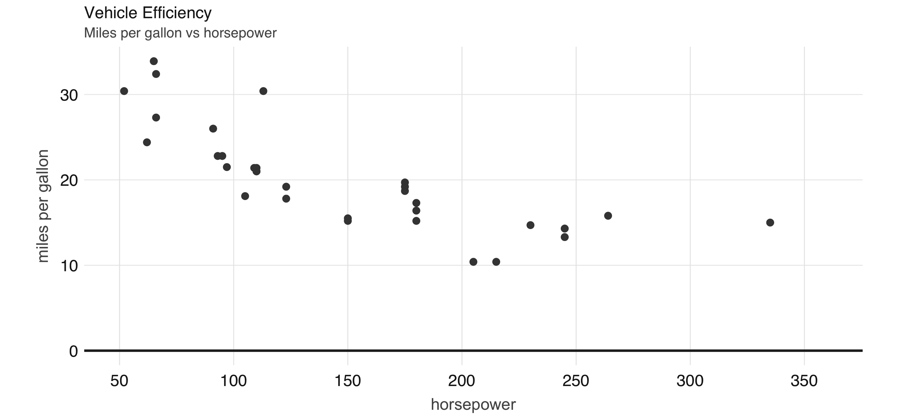 FIGURE 2.5: Horsepower versus miles per gallon
The plot in Figure 2.5, shows that as we increase the horsepower in a vehicle, its fuel efficiency measured in miles per gallon decreases.
Although this is insightful, it’s difficult to predict numerically how increased horsepower would affect fuel efficiency.
Modeling can help us overcome this.
FIGURE 2.5: Horsepower versus miles per gallon
The plot in Figure 2.5, shows that as we increase the horsepower in a vehicle, its fuel efficiency measured in miles per gallon decreases.
Although this is insightful, it’s difficult to predict numerically how increased horsepower would affect fuel efficiency.
Modeling can help us overcome this.
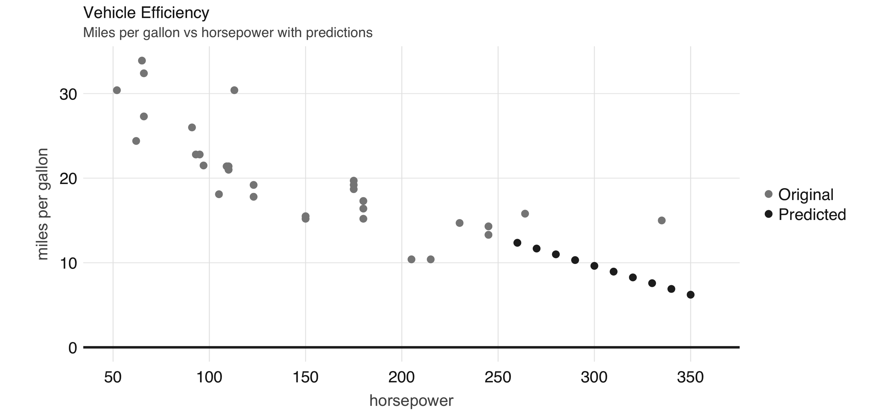 FIGURE 2.6: Horsepower versus miles per gallon with predictions
Even though the previous example lacks many of the appropriate techniques that you should use while modeling, it’s also a simple example to briefly introduce the modeling capabilities of Spark.
We introduce all of the Spark models, techniques, and best practices in Chapter 4.
FIGURE 2.6: Horsepower versus miles per gallon with predictions
Even though the previous example lacks many of the appropriate techniques that you should use while modeling, it’s also a simple example to briefly introduce the modeling capabilities of Spark.
We introduce all of the Spark models, techniques, and best practices in Chapter 4.
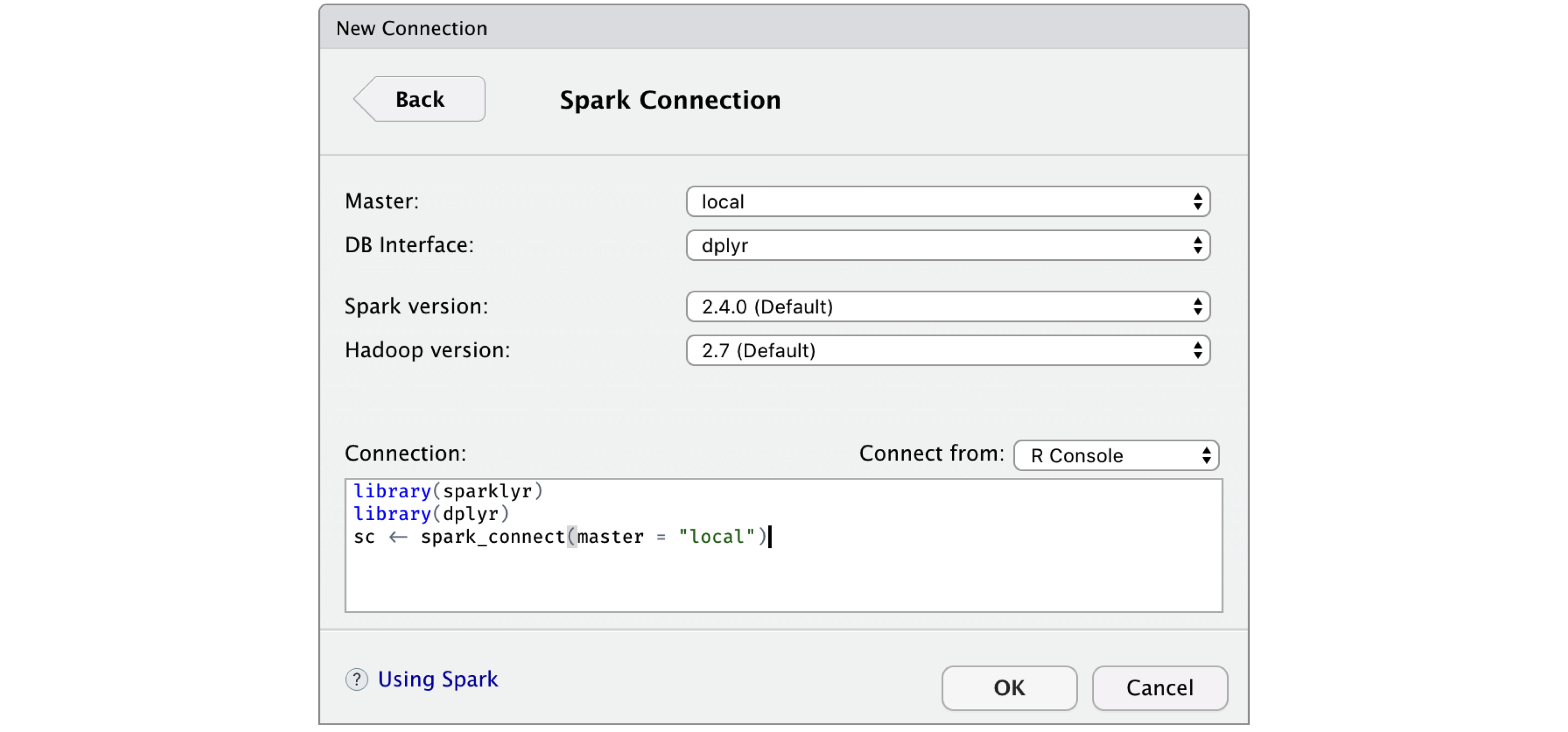 FIGURE 2.7: RStudio New Spark Connection dialog
After you’re connected to Spark, RStudio displays your available datasets in the Connections tab, as shown in Figure 2.8.
This is a useful way to track your existing datasets and provides an easy way to explore each of them.
FIGURE 2.7: RStudio New Spark Connection dialog
After you’re connected to Spark, RStudio displays your available datasets in the Connections tab, as shown in Figure 2.8.
This is a useful way to track your existing datasets and provides an easy way to explore each of them.
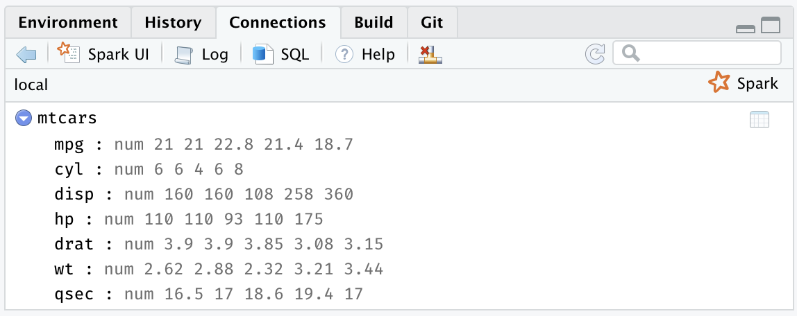 FIGURE 2.8: The RStudio Connections tab
Additionally, an active connection provides the following custom actions:
FIGURE 2.8: The RStudio Connections tab
Additionally, an active connection provides the following custom actions:
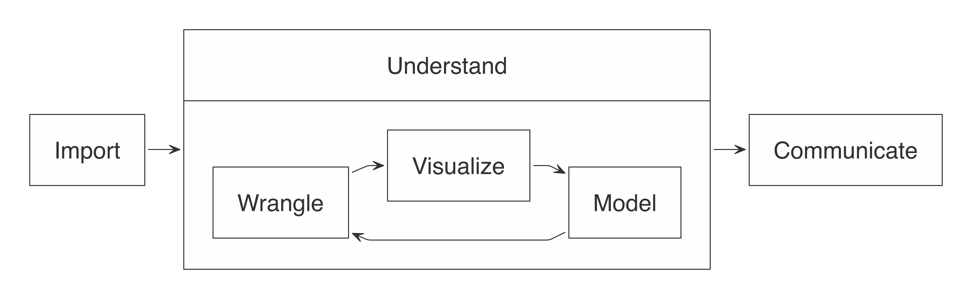 FIGURE 3.1: The general steps of a data analysis
When working with not-large-scale datasets—as in datasets that fit in memory—we can perform all those steps from R, without using Spark.
However, when data does not fit in memory or computation is simply too slow, we can slightly modify this approach by incorporating Spark.
But how?
For data analysis, the ideal approach is to let Spark do what it’s good at.
Spark is a(((“parallel execution”))) parallel computation engine that works at a large scale and provides a SQL engine and modeling libraries.
You can use these to perform most of the same operations R performs.
Such operations include data selection, transformation, and modeling.
Additionally, Spark includes tools for performing specialized computational work like graph analysis, stream processing, and many others.
For now, we will skip those non-rectangular datasets and present them in later chapters.
You can perform data import, wrangling, and modeling within Spark.
You can also partly do visualization with Spark, which we cover later in this chapter.
The idea is to use R to tell Spark what data operations to run, and then only bring the results into R.
As illustrated in Figure 3.2, the ideal method pushes compute to the Spark cluster and then collects results into R.
FIGURE 3.1: The general steps of a data analysis
When working with not-large-scale datasets—as in datasets that fit in memory—we can perform all those steps from R, without using Spark.
However, when data does not fit in memory or computation is simply too slow, we can slightly modify this approach by incorporating Spark.
But how?
For data analysis, the ideal approach is to let Spark do what it’s good at.
Spark is a(((“parallel execution”))) parallel computation engine that works at a large scale and provides a SQL engine and modeling libraries.
You can use these to perform most of the same operations R performs.
Such operations include data selection, transformation, and modeling.
Additionally, Spark includes tools for performing specialized computational work like graph analysis, stream processing, and many others.
For now, we will skip those non-rectangular datasets and present them in later chapters.
You can perform data import, wrangling, and modeling within Spark.
You can also partly do visualization with Spark, which we cover later in this chapter.
The idea is to use R to tell Spark what data operations to run, and then only bring the results into R.
As illustrated in Figure 3.2, the ideal method pushes compute to the Spark cluster and then collects results into R.
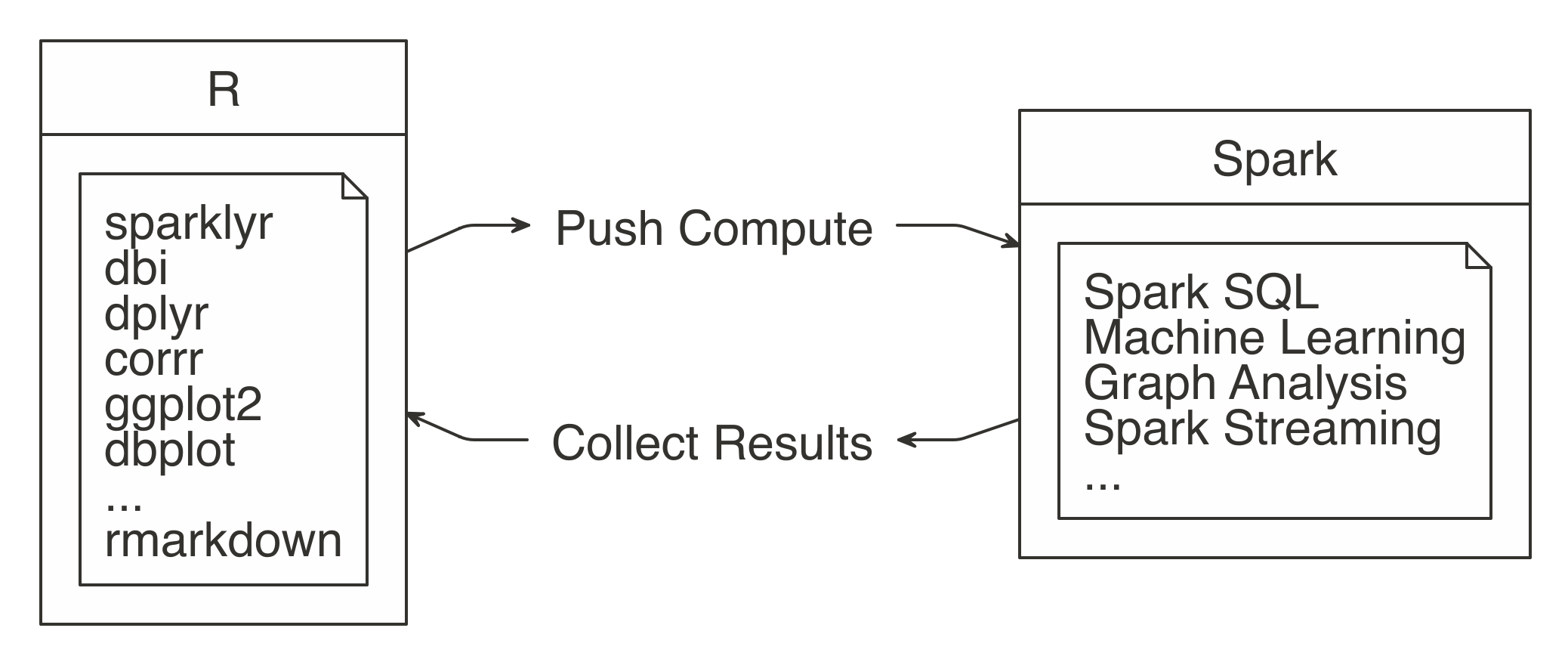 FIGURE 3.2: Spark computes while R collects results
The
FIGURE 3.2: Spark computes while R collects results
The 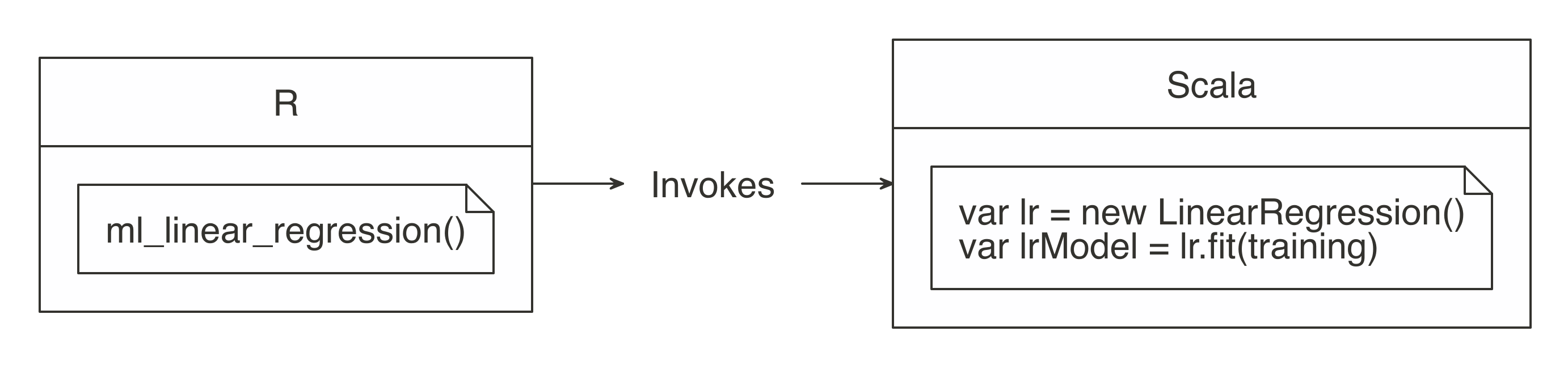 FIGURE 3.3: R functions call Spark functionality
For more common data manipulation tasks,
FIGURE 3.3: R functions call Spark functionality
For more common data manipulation tasks,  FIGURE 3.4: dplyr writes SQL in Spark
To practice as you learn, the rest of this chapter’s code uses a single exercise that runs in the local Spark master.
This way, you can replicate the code on your personal computer.
Make sure
FIGURE 3.4: dplyr writes SQL in Spark
To practice as you learn, the rest of this chapter’s code uses a single exercise that runs in the local Spark master.
This way, you can replicate the code on your personal computer.
Make sure 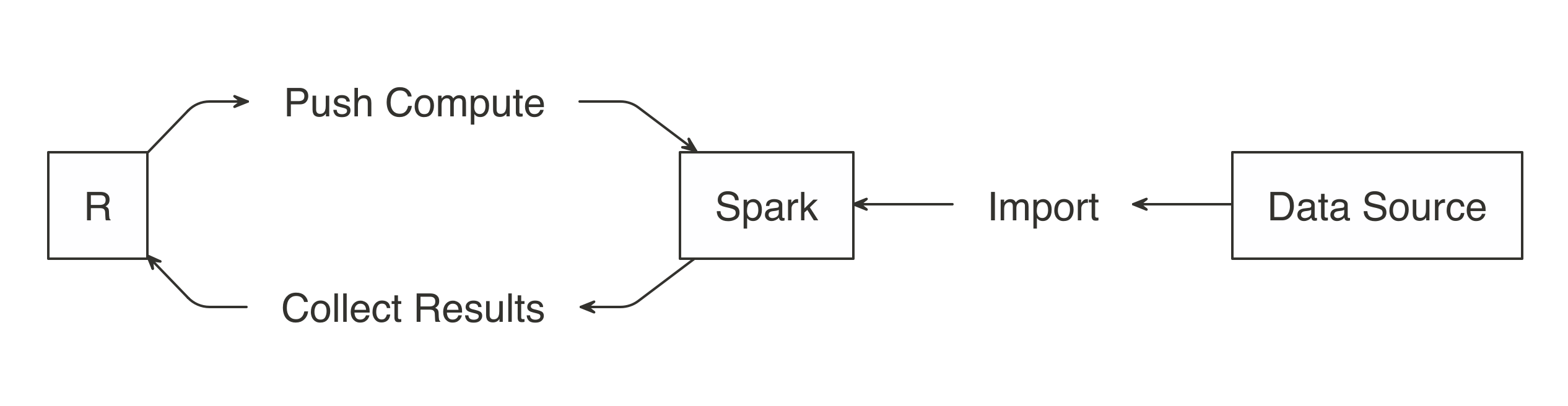 FIGURE 3.5: Import data to Spark not R
Note: When you’re performing analysis over large-scale datasets, the vast majority of the necessary data will already be available in your Spark cluster (which is usually made available to users via Hive tables or by accessing the file system directly).
Chapter 8 will cover this extensively.
Rather than importing all data into Spark, you can request Spark to access the data source without importing it—this is a decision you should make based on speed and performance.
Importing all of the data into the Spark session incurs a one-time up-front cost, since Spark needs to wait for the data to be loaded before analyzing it.
If the data is not imported, you usually incur a cost with every Spark operation since Spark needs to retrieve a subset from the cluster’s storage, which is usually disk drives that happen to be much slower than reading from Spark’s memory.
More on this topic will be covered in Chapter 9.
Let’s prime the session with some data by importing
FIGURE 3.5: Import data to Spark not R
Note: When you’re performing analysis over large-scale datasets, the vast majority of the necessary data will already be available in your Spark cluster (which is usually made available to users via Hive tables or by accessing the file system directly).
Chapter 8 will cover this extensively.
Rather than importing all data into Spark, you can request Spark to access the data source without importing it—this is a decision you should make based on speed and performance.
Importing all of the data into the Spark session incurs a one-time up-front cost, since Spark needs to wait for the data to be loaded before analyzing it.
If the data is not imported, you usually incur a cost with every Spark operation since Spark needs to retrieve a subset from the cluster’s storage, which is usually disk drives that happen to be much slower than reading from Spark’s memory.
More on this topic will be covered in Chapter 9.
Let’s prime the session with some data by importing 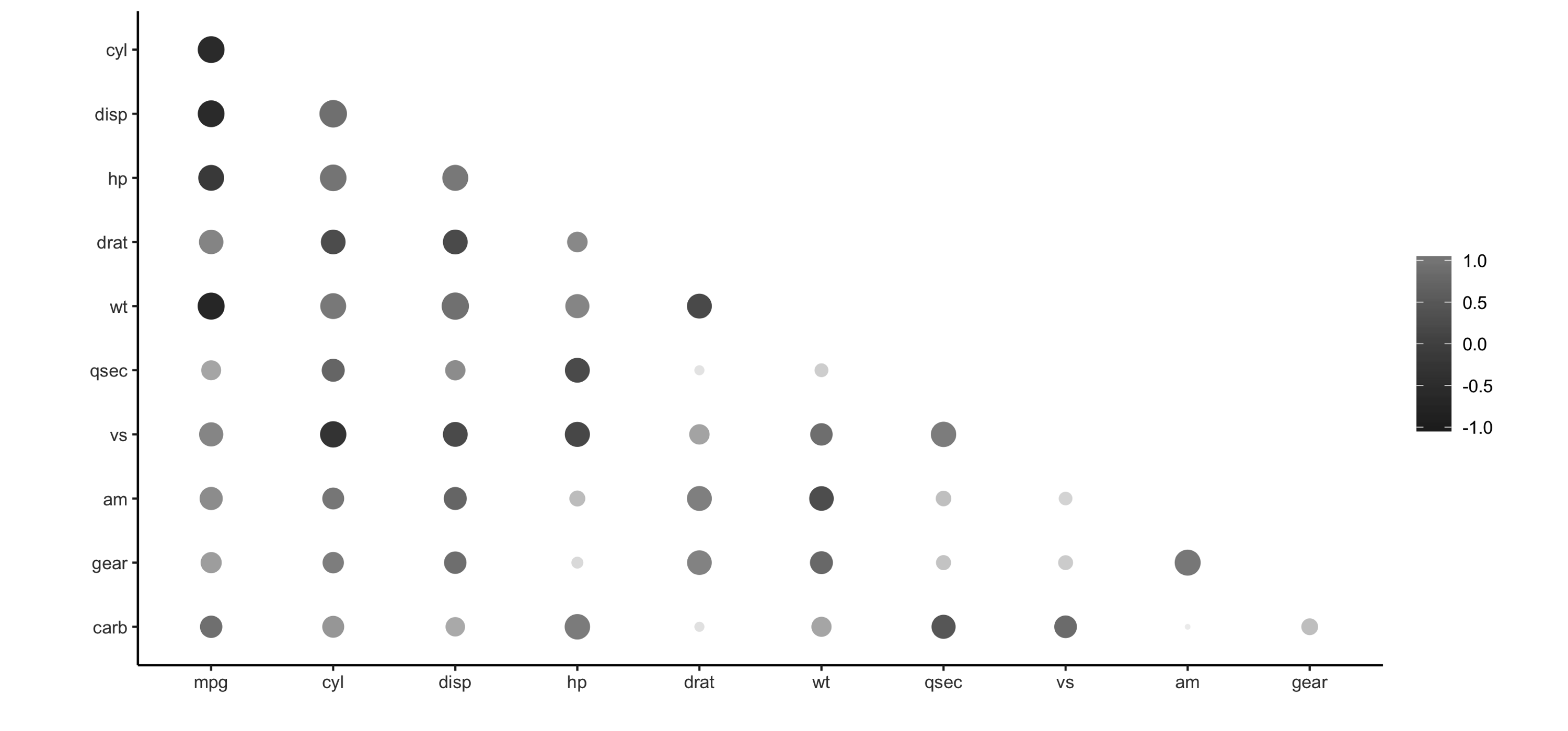 FIGURE 3.6: Using rplot() to visualize correlations
It is much easier to see which relationships are positive or negative: positive relationships are in gray, and negative relationships are black.
The size of the circle indicates how significant their relationship is.
The power of visualizing data is in how much easier it makes it for us to understand results.
The next section expands on this step of the process.
FIGURE 3.6: Using rplot() to visualize correlations
It is much easier to see which relationships are positive or negative: positive relationships are in gray, and negative relationships are black.
The size of the circle indicates how significant their relationship is.
The power of visualizing data is in how much easier it makes it for us to understand results.
The next section expands on this step of the process.
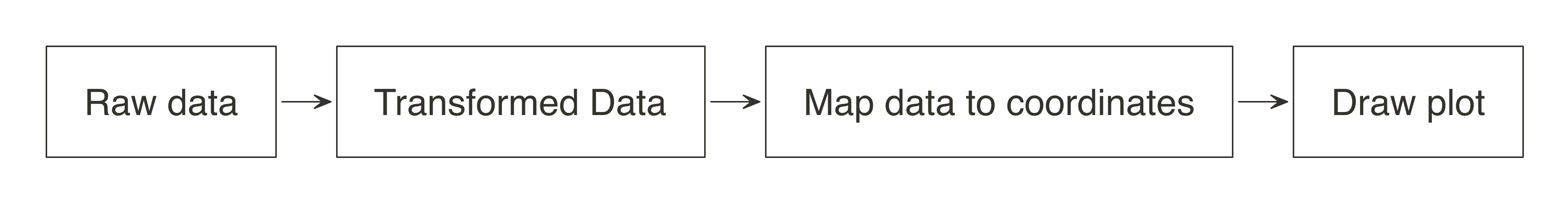 FIGURE 3.7: Stages of an R plot
In essence, the approach for visualizing is the same as in wrangling: push the computation to Spark, and then collect the results in R for plotting.
As illustrated in Figure 3.8, the heavy lifting of preparing the data, such as aggregating the data by groups or bins, can be done within Spark, and then the much smaller dataset can be collected into R.
Inside R, the plot becomes a more basic operation.
For example, for a histogram, the bins are calculated in Spark, and then plotted in R using a simple column plot, as opposed to a histogram plot, because there is no need for R to recalculate the bins.
FIGURE 3.7: Stages of an R plot
In essence, the approach for visualizing is the same as in wrangling: push the computation to Spark, and then collect the results in R for plotting.
As illustrated in Figure 3.8, the heavy lifting of preparing the data, such as aggregating the data by groups or bins, can be done within Spark, and then the much smaller dataset can be collected into R.
Inside R, the plot becomes a more basic operation.
For example, for a histogram, the bins are calculated in Spark, and then plotted in R using a simple column plot, as opposed to a histogram plot, because there is no need for R to recalculate the bins.
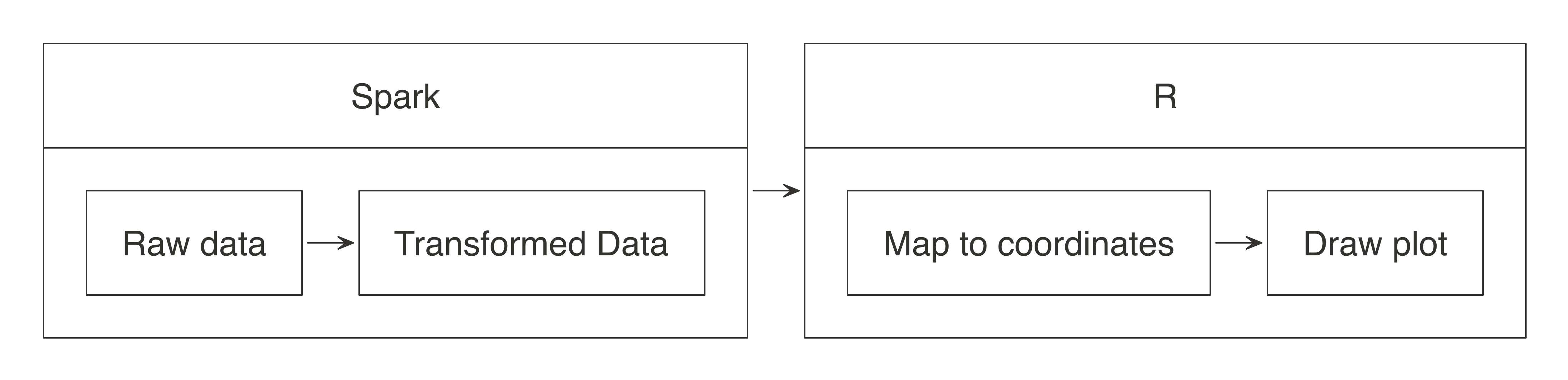 FIGURE 3.8: Plotting with Spark and R
Let’s apply this conceptual model when using
FIGURE 3.8: Plotting with Spark and R
Let’s apply this conceptual model when using  FIGURE 3.9: Plotting inside R
In this case, the
FIGURE 3.9: Plotting inside R
In this case, the 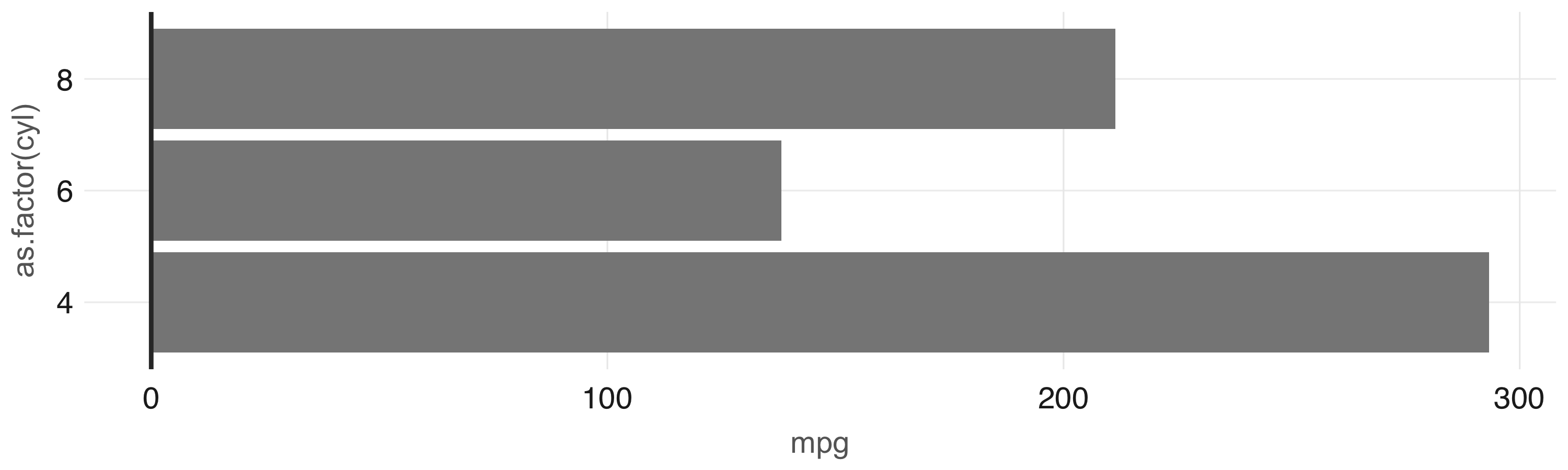 FIGURE 3.10: Plot with aggregation in Spark
Any other
FIGURE 3.10: Plot with aggregation in Spark
Any other 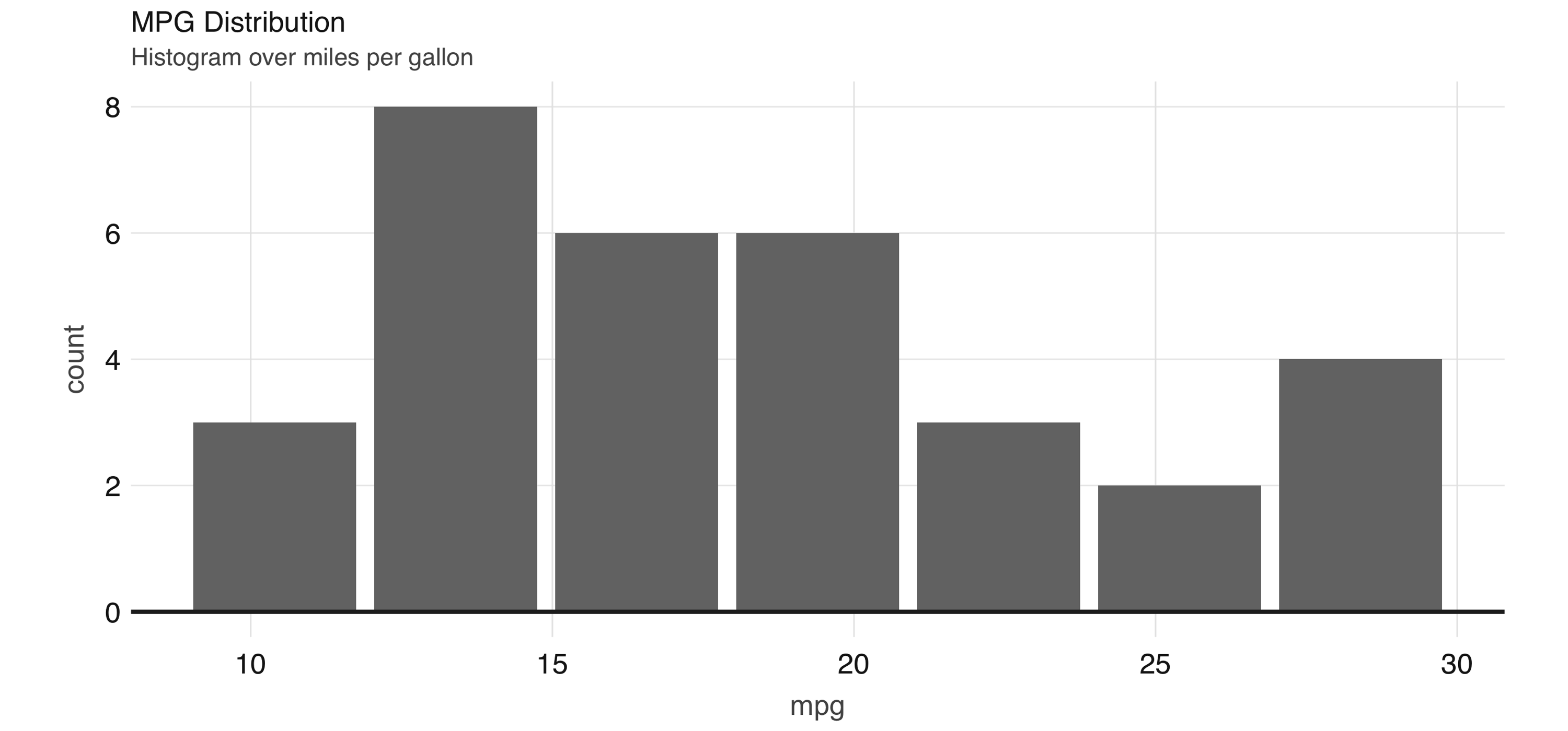 FIGURE 3.11: Histogram created by dbplot
Histograms provide a great way to analyze a single variable.
To analyze two variables, a scatter or raster plot is commonly used.
Scatter plots are used to compare the relationship between two continuous variables.
For example, a scatter plot will display the relationship between the weight of a car and its gas consumption.
The plot in Figure 3.12 shows that the higher the weight, the higher the gas consumption because the dots clump together into almost a line that goes from the upper left toward the lower right.
Here’s the code to generate the plot:
FIGURE 3.11: Histogram created by dbplot
Histograms provide a great way to analyze a single variable.
To analyze two variables, a scatter or raster plot is commonly used.
Scatter plots are used to compare the relationship between two continuous variables.
For example, a scatter plot will display the relationship between the weight of a car and its gas consumption.
The plot in Figure 3.12 shows that the higher the weight, the higher the gas consumption because the dots clump together into almost a line that goes from the upper left toward the lower right.
Here’s the code to generate the plot:
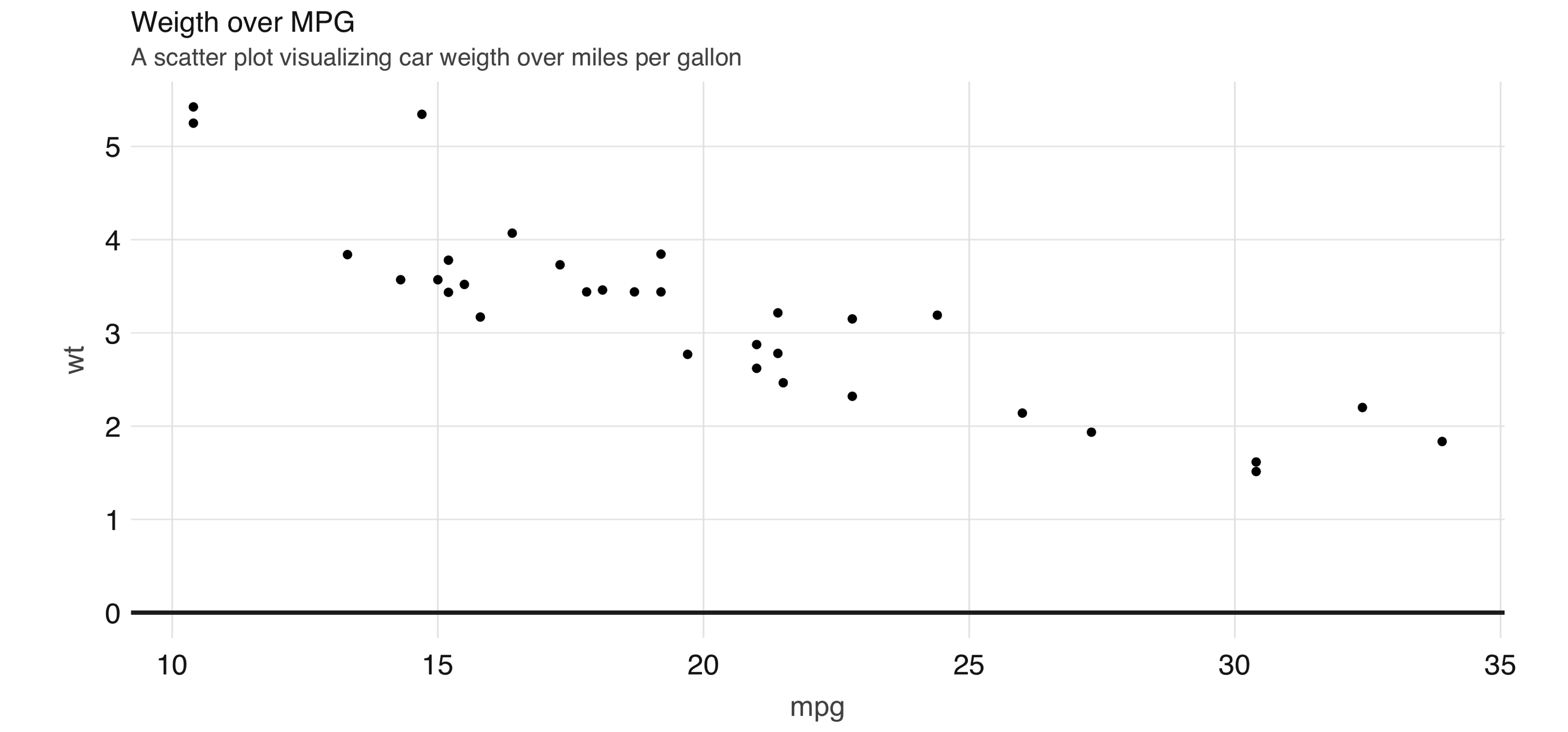 FIGURE 3.12: Scatter plot example in Spark
However, for scatter plots, no amount of “pushing the computation” to Spark will help with this problem because the data must be plotted in individual dots.
The best alternative is to find a plot type that represents the x/y relationship and concentration in a way that it is easy to perceive and to “physically” plot.
The raster plot might be the best answer.
A raster plot returns a grid of x/y positions and the results of a given aggregation, usually represented by the color of the square.
You can use
FIGURE 3.12: Scatter plot example in Spark
However, for scatter plots, no amount of “pushing the computation” to Spark will help with this problem because the data must be plotted in individual dots.
The best alternative is to find a plot type that represents the x/y relationship and concentration in a way that it is easy to perceive and to “physically” plot.
The raster plot might be the best answer.
A raster plot returns a grid of x/y positions and the results of a given aggregation, usually represented by the color of the square.
You can use 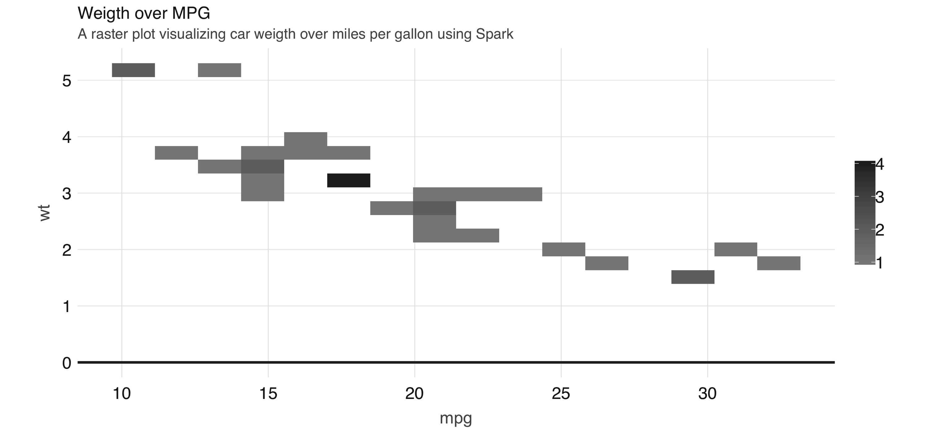 FIGURE 3.13: A raster plot using Spark
As shown in 3.13, the resulting plot returns a grid no bigger than 5 x 5.
This limits the number of records that need to be collected into R to 25.
Tip: You can also use
FIGURE 3.13: A raster plot using Spark
As shown in 3.13, the resulting plot returns a grid no bigger than 5 x 5.
This limits the number of records that need to be collected into R to 25.
Tip: You can also use  FIGURE 3.14: R Markdown HTML output
You can now easily share this report, and viewers of won’t need Spark or R to read and consume its contents; it’s just a self-contained HTML file, trivial to open in any browser.
It is also common to distill insights of a report into many other output formats.
Switching is quite easy: in the top frontmatter, change the
FIGURE 3.14: R Markdown HTML output
You can now easily share this report, and viewers of won’t need Spark or R to read and consume its contents; it’s just a self-contained HTML file, trivial to open in any browser.
It is also common to distill insights of a report into many other output formats.
Switching is quite easy: in the top frontmatter, change the 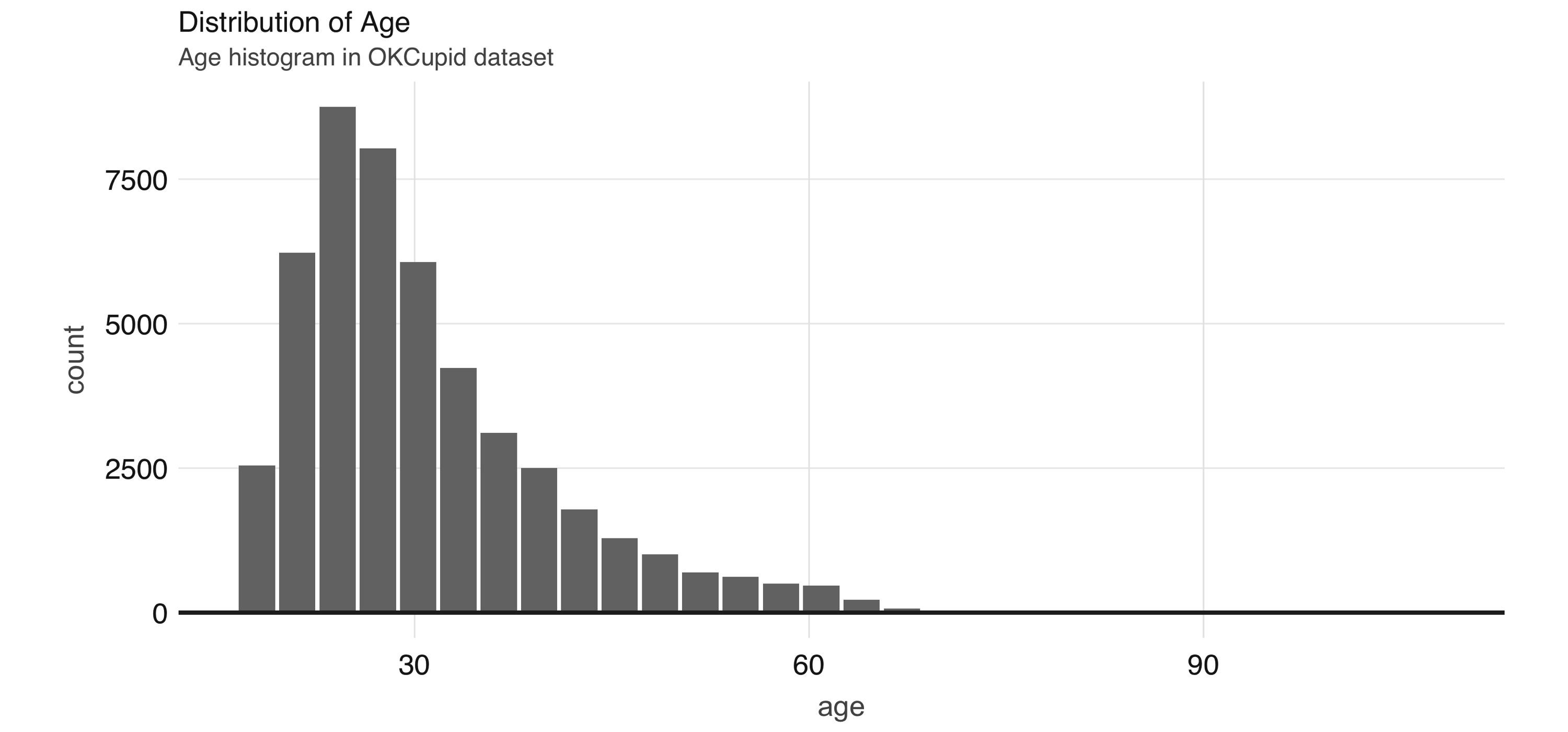 FIGURE 4.1: Distribution of age
A common EDA exercise is to look at the relationships between the response and the individual predictors.
Often, you might have prior business knowledge of what these relationships should be, so this can serve as a data quality check.
Also, unexpected trends can inform variable interactions that you might want to include in the model.
As an example, we can explore the
FIGURE 4.1: Distribution of age
A common EDA exercise is to look at the relationships between the response and the individual predictors.
Often, you might have prior business knowledge of what these relationships should be, so this can serve as a data quality check.
Also, unexpected trends can inform variable interactions that you might want to include in the model.
As an example, we can explore the 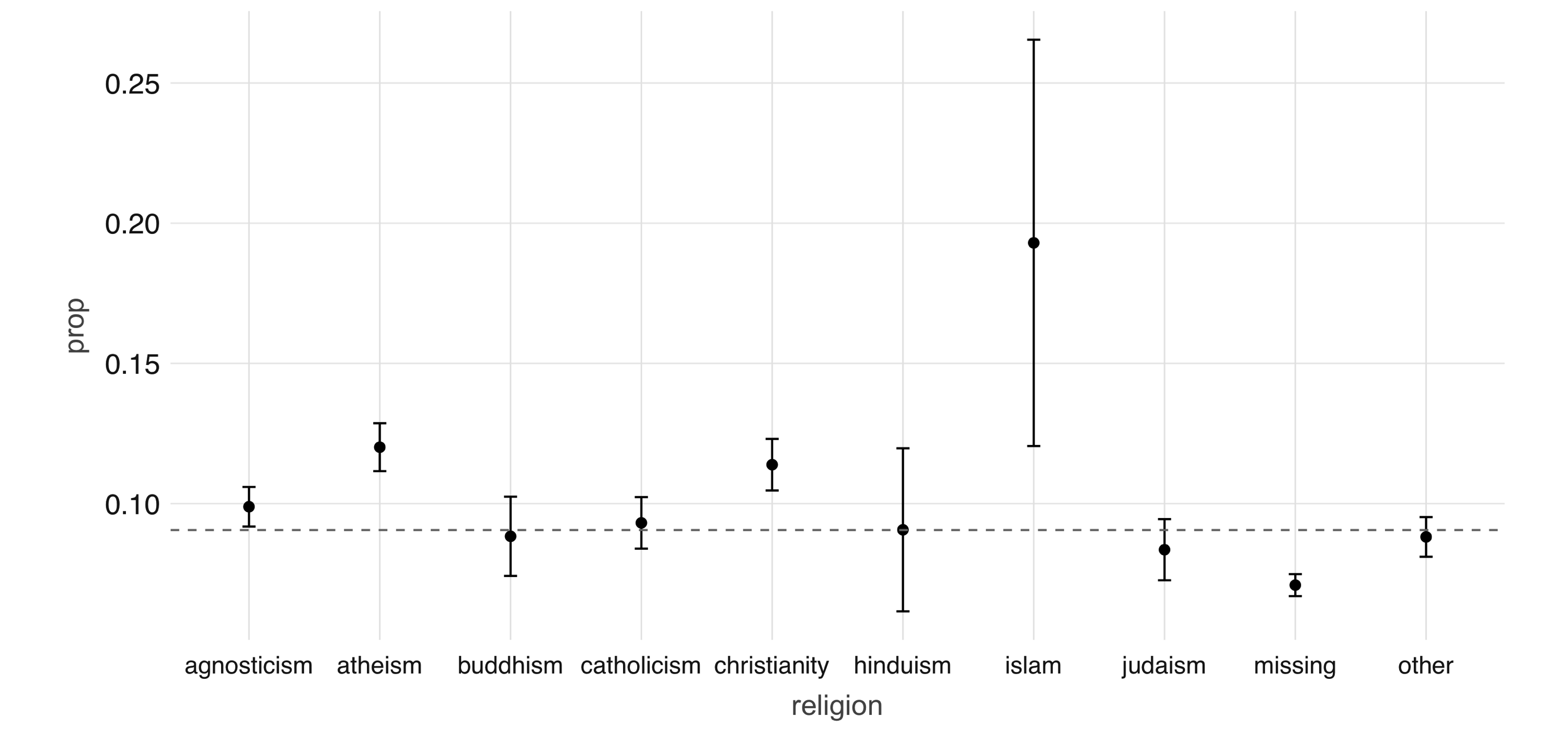 FIGURE 4.2: Proportion of individuals not currently employed, by religion
Next, we take a look at the relationship between a couple of predictors: alcohol use and drug use.
We would expect there to be some correlation between them.
You can compute a contingency table via
FIGURE 4.2: Proportion of individuals not currently employed, by religion
Next, we take a look at the relationship between a couple of predictors: alcohol use and drug use.
We would expect there to be some correlation between them.
You can compute a contingency table via 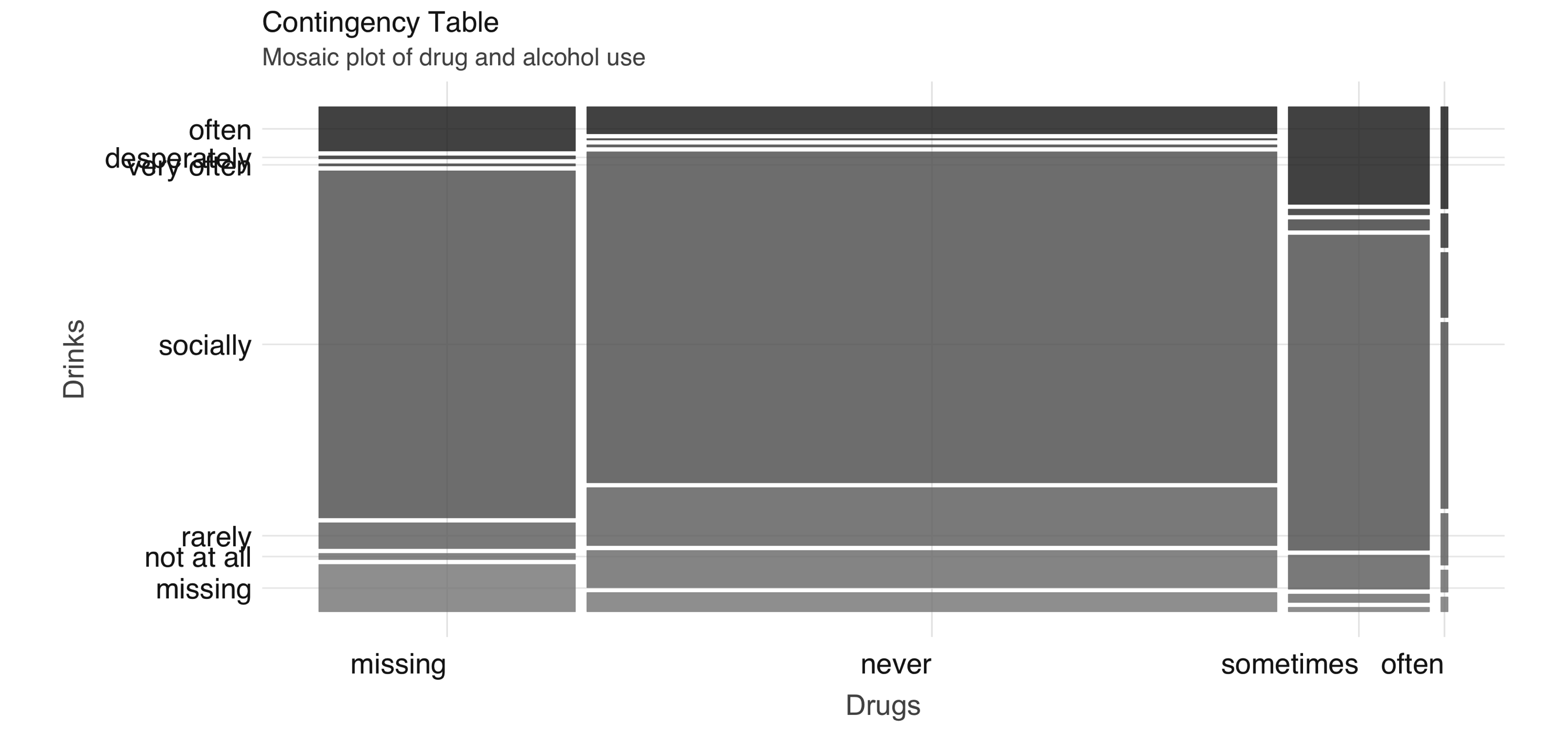 FIGURE 4.3: Mosaic plot of drug and alcohol use
To further explore the relationship between these two variables, we can perform correspondence analysis18 using the
FIGURE 4.3: Mosaic plot of drug and alcohol use
To further explore the relationship between these two variables, we can perform correspondence analysis18 using the 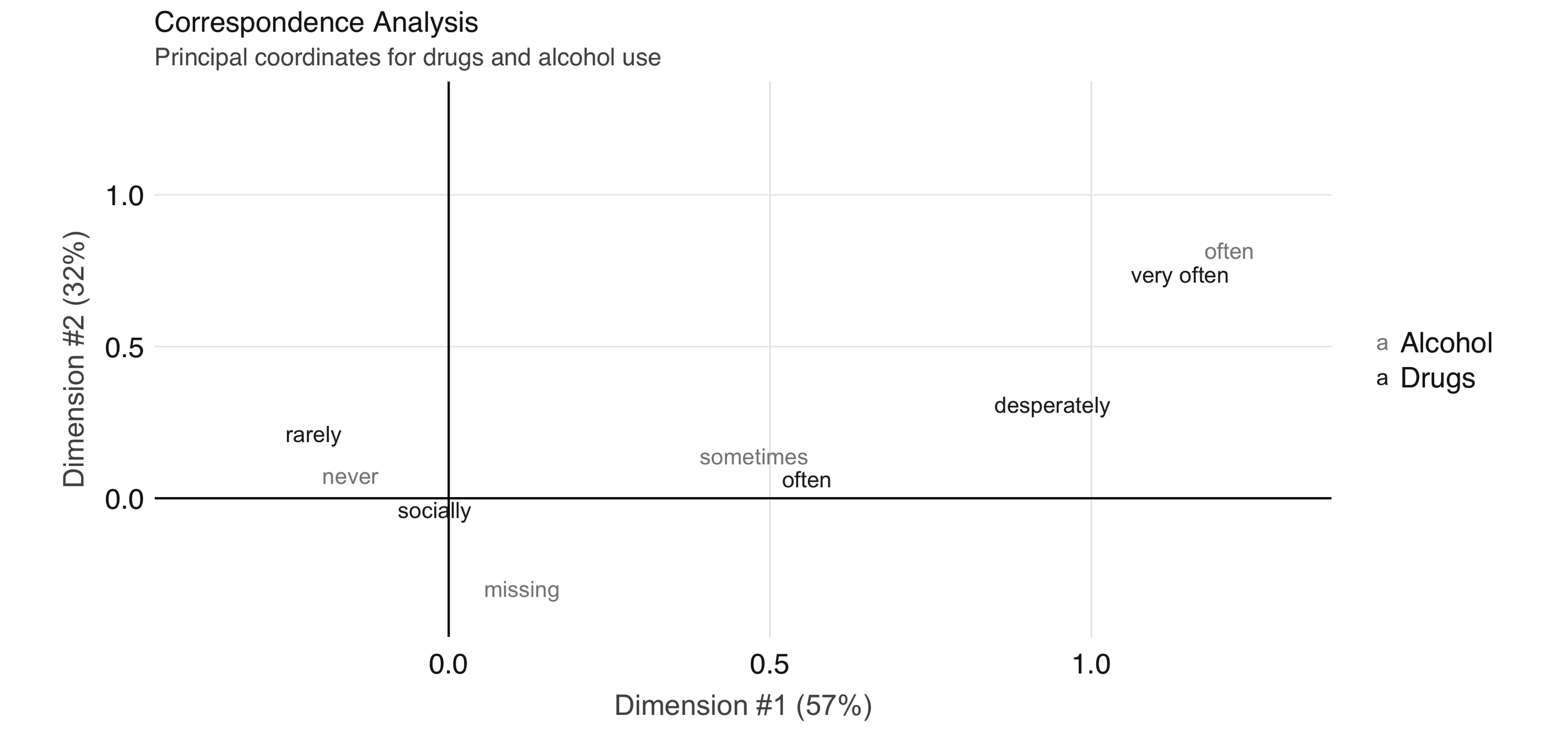 FIGURE 4.4: Correspondence analysis principal coordinates for drug and alcohol use
In Figure 4.4, we see that the correspondence analysis procedure has transformed the factors into variables called principal coordinates, which correspond to the axes in the plot and represent how much information in the contingency table they contain.
We can, for example, interpret the proximity of “drinking often” and “using drugs very often” as indicating association.
This concludes our discussion on EDA.
Let’s proceed to feature engineering.
FIGURE 4.4: Correspondence analysis principal coordinates for drug and alcohol use
In Figure 4.4, we see that the correspondence analysis procedure has transformed the factors into variables called principal coordinates, which correspond to the axes in the plot and represent how much information in the contingency table they contain.
We can, for example, interpret the proximity of “drinking often” and “using drugs very often” as indicating association.
This concludes our discussion on EDA.
Let’s proceed to feature engineering.
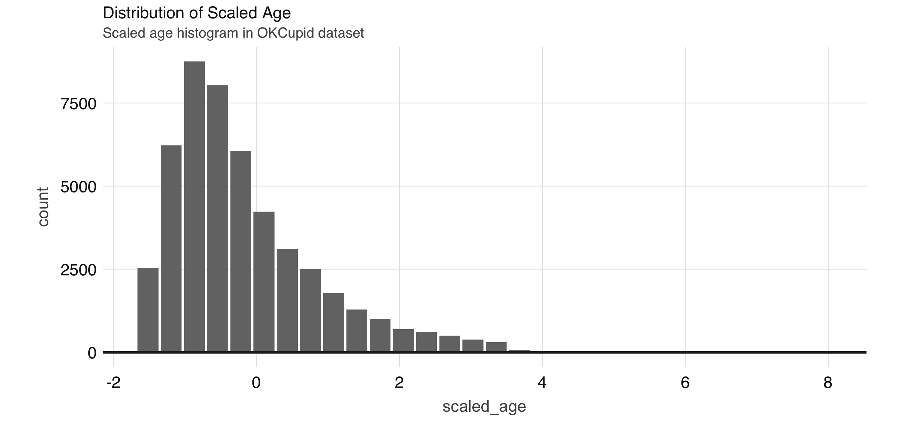 FIGURE 4.5: Distribution of scaled age
Since some of the profile features are multiple-select—in other words, a person can choose to associate multiple options for a variable—we need to process them before we can build meaningful models.
If we take a look at the ethnicity column, for example, we see that there are many different combinations:
FIGURE 4.5: Distribution of scaled age
Since some of the profile features are multiple-select—in other words, a person can choose to associate multiple options for a variable—we need to process them before we can build meaningful models.
If we take a look at the ethnicity column, for example, we see that there are many different combinations:
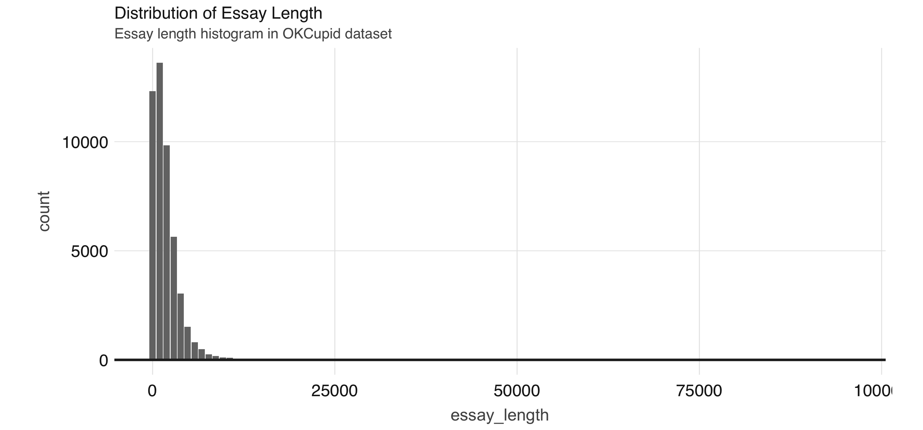 FIGURE 4.6: Distribution of essay length
We use this dataset in Chapter 5, so let’s save it first as a Parquet file—an efficient file format ideal for numeric data:
FIGURE 4.6: Distribution of essay length
We use this dataset in Chapter 5, so let’s save it first as a Parquet file—an efficient file format ideal for numeric data:
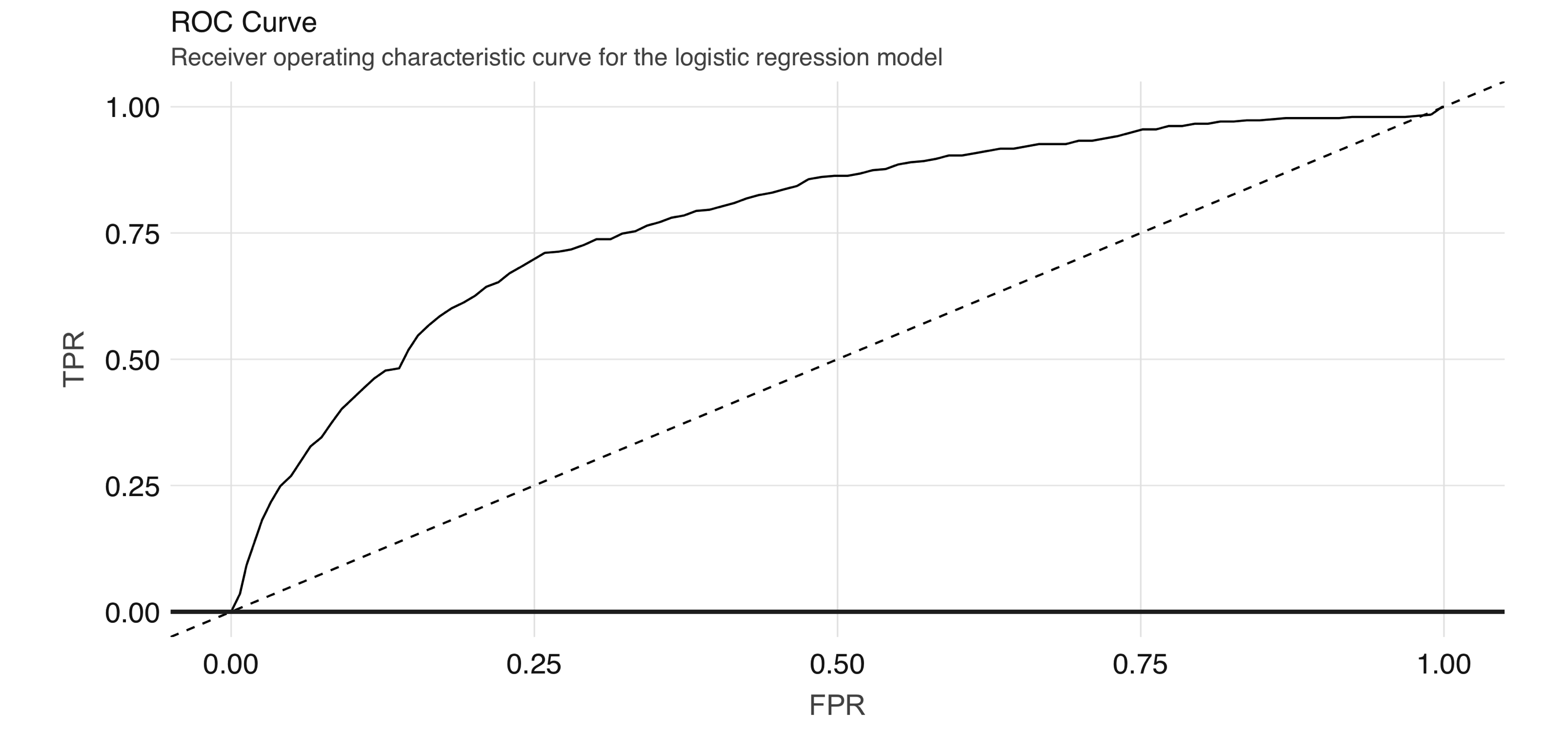 FIGURE 4.7: ROC curve for the logistic regression model
The ROC curve plots the true positive rate (sensitivity) against the false positive rate (1–specificity) for varying values of the classification threshold.
In practice, the business problem helps to determine where on the curve one sets the threshold for classification.
The AUC is a summary measure for determining the quality of a model, and we can compute it by calling the
FIGURE 4.7: ROC curve for the logistic regression model
The ROC curve plots the true positive rate (sensitivity) against the false positive rate (1–specificity) for varying values of the classification threshold.
In practice, the business problem helps to determine where on the curve one sets the threshold for classification.
The AUC is a summary measure for determining the quality of a model, and we can compute it by calling the 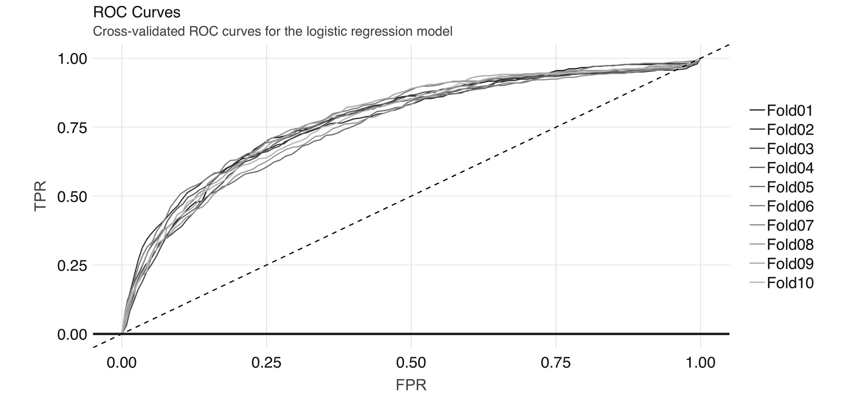 FIGURE 4.8: Cross-validated ROC curves for the logistic regression model
And we can obtain the average AUC metric:
FIGURE 4.8: Cross-validated ROC curves for the logistic regression model
And we can obtain the average AUC metric:
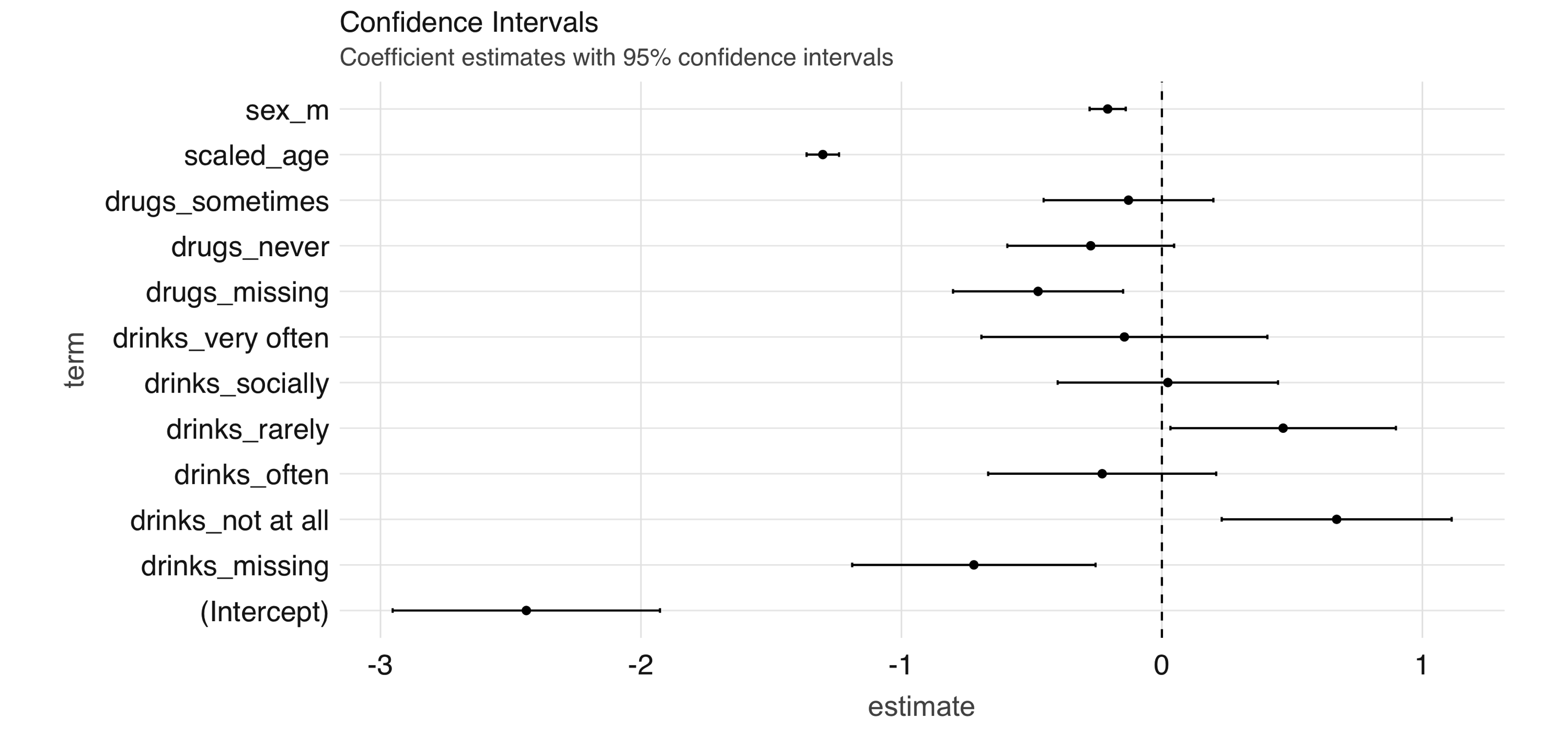 FIGURE 4.9: Coefficient estimates with 95% confidence intervals
Note: Both
FIGURE 4.9: Coefficient estimates with 95% confidence intervals
Note: Both 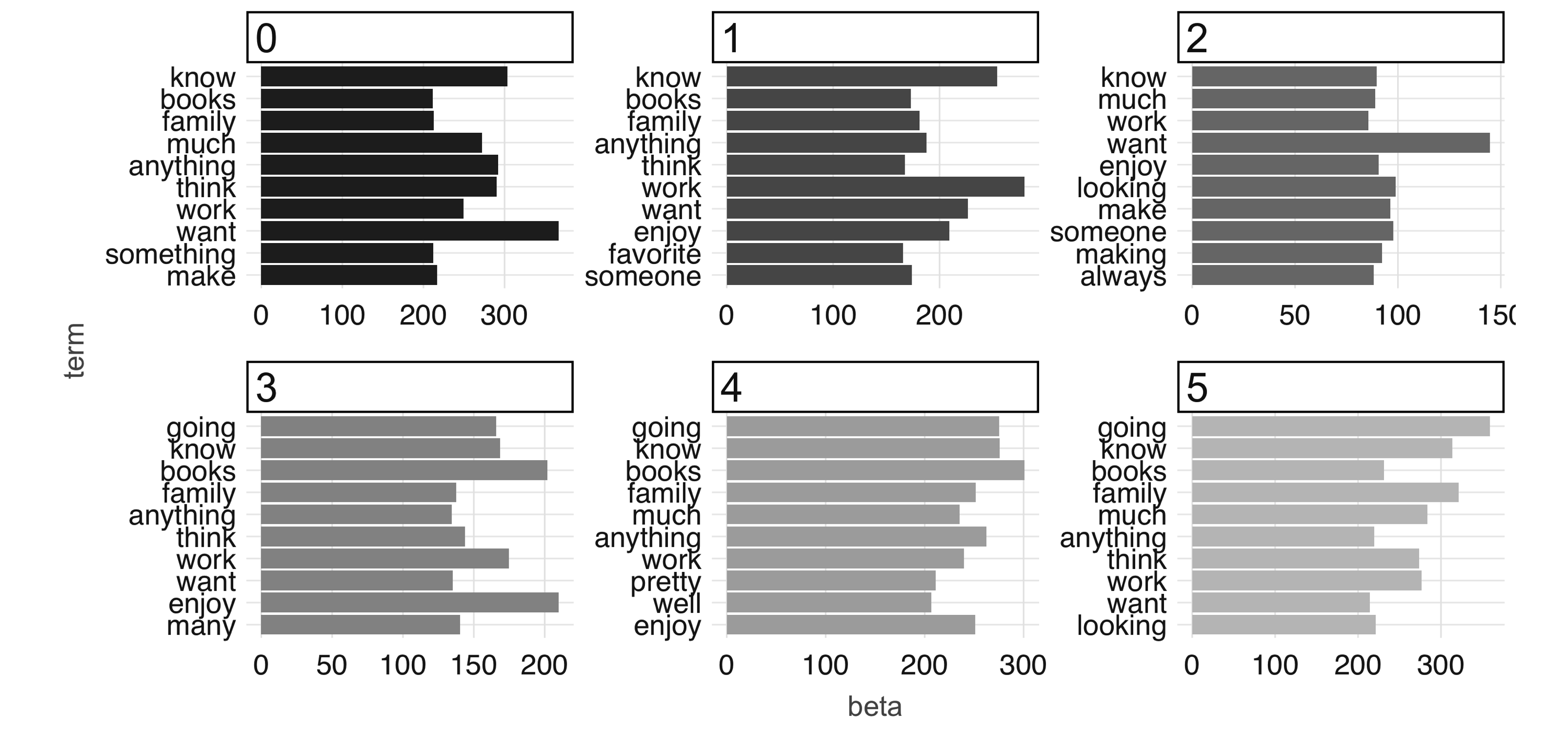 FIGURE 4.10: The most common terms per topic in the first iteration
At 100 iterations, we can see “topics” starting to emerge.
This could be interesting information in its own right if you were digging into a large collection of documents with which you aren’t familiar.
The learned topics can also serve as features in a downstream supervised learning task; for example, we could consider using the topic number as a predictor in our model to predict employment status in our predictive modeling example.
FIGURE 4.10: The most common terms per topic in the first iteration
At 100 iterations, we can see “topics” starting to emerge.
This could be interesting information in its own right if you were digging into a large collection of documents with which you aren’t familiar.
The learned topics can also serve as features in a downstream supervised learning task; for example, we could consider using the topic number as a predictor in our model to predict employment status in our predictive modeling example.
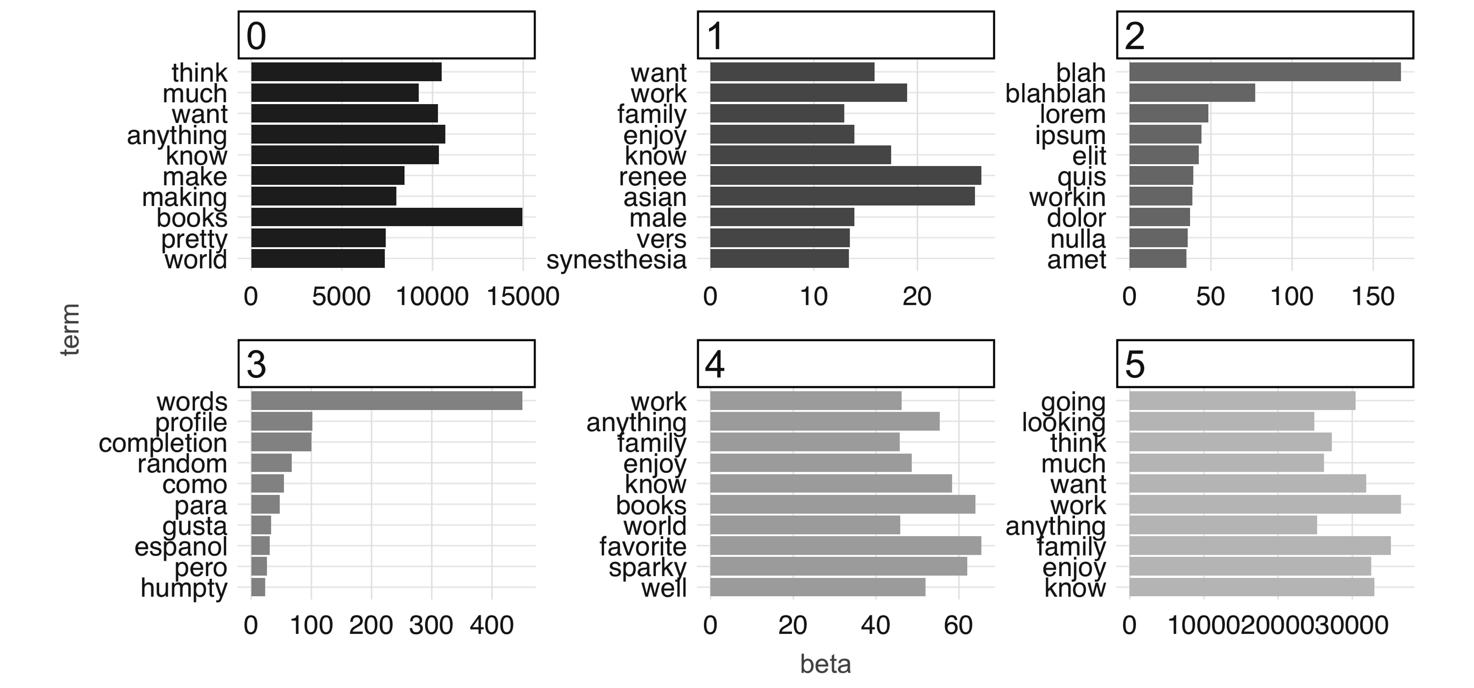 FIGURE 4.11: The most common terms per topic after 100 iterations
Finally, to conclude this chapter you should disconnect from Spark.
Chapter 5 also makes use of the
FIGURE 4.11: The most common terms per topic after 100 iterations
Finally, to conclude this chapter you should disconnect from Spark.
Chapter 5 also makes use of the 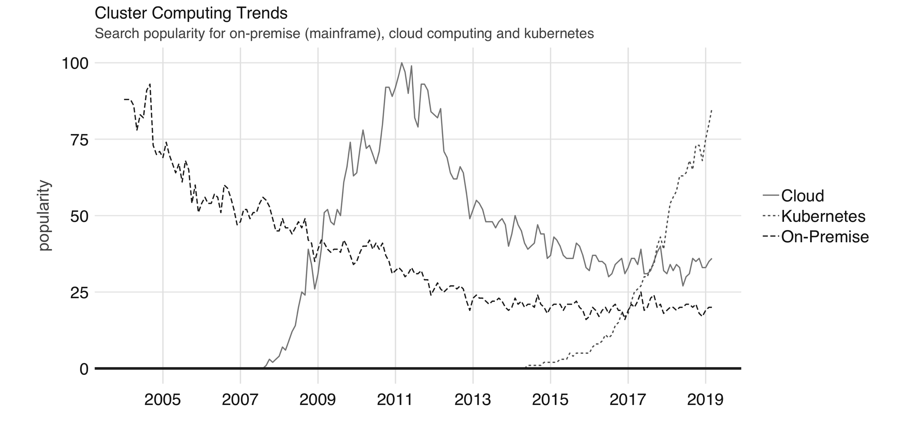 FIGURE 6.1: Google trends for on-premises (mainframe), cloud computing, and Kubernetes
When purchasing hundreds or thousands of computing instances, it doesn’t make sense to keep them in the usual computing case that we are all familiar with; instead, it makes sense to stack them as efficiently as possible on top of one another to minimize the space the use.
This group of efficiently stacked computing instances is known as a rack.
After a cluster grows to thousands of computers, you will also need to host hundreds of racks of computing devices; at this scale, you would also need significant physical space to host those racks.
A building that provides racks of computing instances is usually known as a datacenter.
At the scale of a datacenter, you would also need to find ways to make the building more efficient, especially the cooling system, power supplies, network connectivity, and so on.
Since this is time-consuming, a few organizations have come together to open source their infrastructure under the Open Compute Project initiative, which provides a set of datacenter blueprints free for anyone to use.
There is nothing preventing you from building our own datacenter, and, in fact, many organizations have followed this path.
For instance, Amazon started as an online bookstore, but over the years it grew to sell much more than just books.
Along with its online store growth, its datacenters also grew in size.
In 2002, Amazon considered renting servers in their datacenters to the public, and two years later, Amazon Web Services (AWS) launched as a way to let anyone rent servers in the company’s datacenters on demand, meaning that you did not need to purchase, configure, maintain, or tear down your own clusters; rather, you could rent them directly from AWS.
This on-demand compute model is what we know today as cloud computing.
In the cloud, the cluster you use is not owned by you, and it’s not in your physical building; instead it’s a datacenter owned and managed by someone else.
Today, there are many cloud providers in this space, including AWS, Databricks, Google, Microsoft, Qubole, and many others.
Most cloud computing platforms provide a user interface through either a web application or command line to request and manage resources.
While the benefits of processing data in the cloud were obvious for many years, picking a cloud provider had the unintended side effect of locking in organizations with one particular provider, making it hard to switch between providers or back to on-premises clusters.
Kubernetes, announced by Google in 2014, is an open source system for managing containerized applications across multiple hosts.
In practice, it makes it easier to deploy across multiple cloud providers and on-premises as well.
In summary, we have seen a transition from on-premises to cloud computing and, more recently, Kubernetes.
These technologies are often loosely described as the private cloud, the public cloud, and as one of the orchestration services that can enable a hybrid cloud, respectively.
This chapter walks you through each cluster computing trend in the context of Spark and R.
FIGURE 6.1: Google trends for on-premises (mainframe), cloud computing, and Kubernetes
When purchasing hundreds or thousands of computing instances, it doesn’t make sense to keep them in the usual computing case that we are all familiar with; instead, it makes sense to stack them as efficiently as possible on top of one another to minimize the space the use.
This group of efficiently stacked computing instances is known as a rack.
After a cluster grows to thousands of computers, you will also need to host hundreds of racks of computing devices; at this scale, you would also need significant physical space to host those racks.
A building that provides racks of computing instances is usually known as a datacenter.
At the scale of a datacenter, you would also need to find ways to make the building more efficient, especially the cooling system, power supplies, network connectivity, and so on.
Since this is time-consuming, a few organizations have come together to open source their infrastructure under the Open Compute Project initiative, which provides a set of datacenter blueprints free for anyone to use.
There is nothing preventing you from building our own datacenter, and, in fact, many organizations have followed this path.
For instance, Amazon started as an online bookstore, but over the years it grew to sell much more than just books.
Along with its online store growth, its datacenters also grew in size.
In 2002, Amazon considered renting servers in their datacenters to the public, and two years later, Amazon Web Services (AWS) launched as a way to let anyone rent servers in the company’s datacenters on demand, meaning that you did not need to purchase, configure, maintain, or tear down your own clusters; rather, you could rent them directly from AWS.
This on-demand compute model is what we know today as cloud computing.
In the cloud, the cluster you use is not owned by you, and it’s not in your physical building; instead it’s a datacenter owned and managed by someone else.
Today, there are many cloud providers in this space, including AWS, Databricks, Google, Microsoft, Qubole, and many others.
Most cloud computing platforms provide a user interface through either a web application or command line to request and manage resources.
While the benefits of processing data in the cloud were obvious for many years, picking a cloud provider had the unintended side effect of locking in organizations with one particular provider, making it hard to switch between providers or back to on-premises clusters.
Kubernetes, announced by Google in 2014, is an open source system for managing containerized applications across multiple hosts.
In practice, it makes it easier to deploy across multiple cloud providers and on-premises as well.
In summary, we have seen a transition from on-premises to cloud computing and, more recently, Kubernetes.
These technologies are often loosely described as the private cloud, the public cloud, and as one of the orchestration services that can enable a hybrid cloud, respectively.
This chapter walks you through each cluster computing trend in the context of Spark and R.
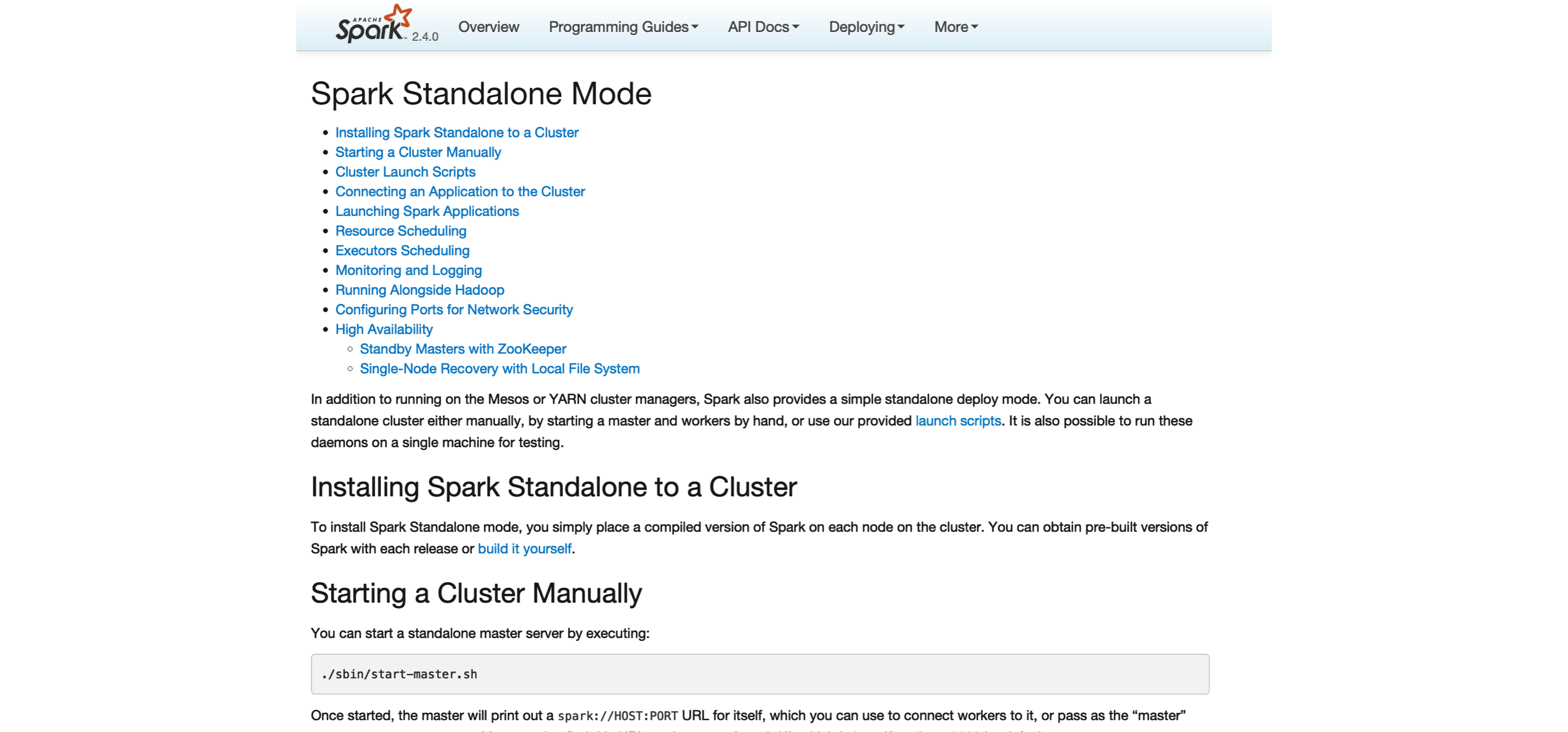 FIGURE 6.2: Spark Standalone website
The previous command initializes the master node.
You can access the master node interface at localhost:8080, as captured in Figure 6.3.
Note that the Spark master URL is specified as spark://address:port; you will need this URL to initialize worker nodes.
We then can initialize a single worker using the master URL; however, you could use a similar approach to initialize multiple workers by running the code multiple times and, potentially, across different machines:
FIGURE 6.2: Spark Standalone website
The previous command initializes the master node.
You can access the master node interface at localhost:8080, as captured in Figure 6.3.
Note that the Spark master URL is specified as spark://address:port; you will need this URL to initialize worker nodes.
We then can initialize a single worker using the master URL; however, you could use a similar approach to initialize multiple workers by running the code multiple times and, potentially, across different machines:
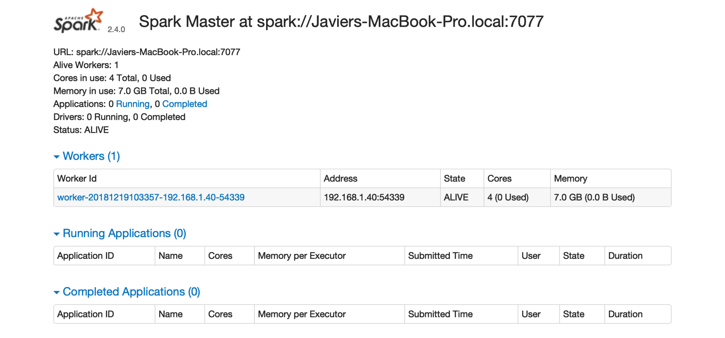 FIGURE 6.3: The Spark Standalone web interface
There is one worker register in Spark Standalone.
Click the link to this worker node to view details for this particular worker, like available memory and cores, as shown in Figure 6.4.
FIGURE 6.3: The Spark Standalone web interface
There is one worker register in Spark Standalone.
Click the link to this worker node to view details for this particular worker, like available memory and cores, as shown in Figure 6.4.
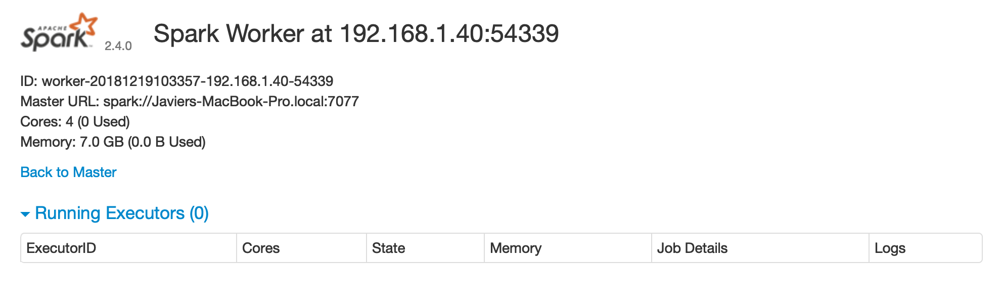 FIGURE 6.4: Spark Standalone worker web interface
After you are done performing computations in this cluster, you will need to stop the master and worker nodes.
You can use the
FIGURE 6.4: Spark Standalone worker web interface
After you are done performing computations in this cluster, you will need to stop the master and worker nodes.
You can use the 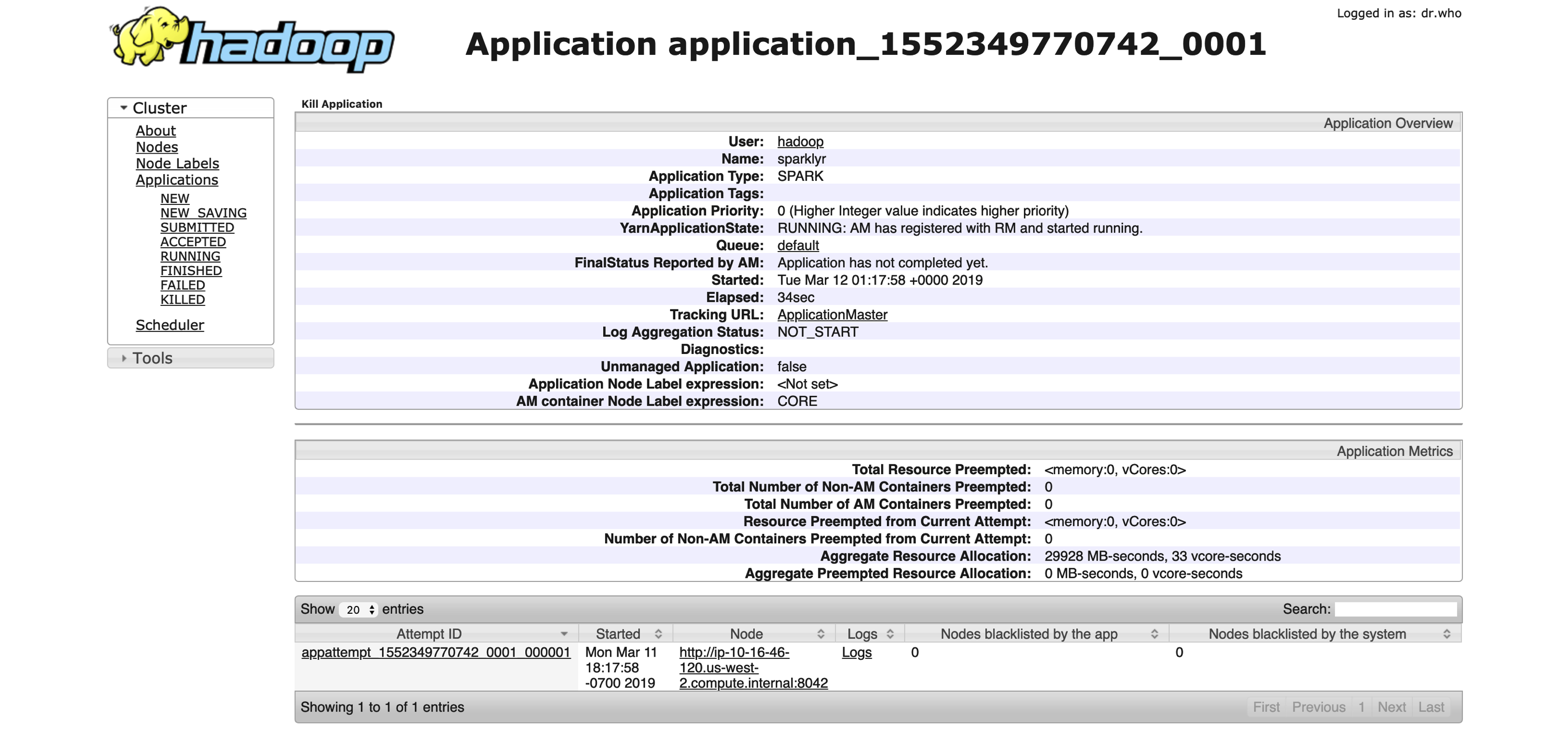 FIGURE 6.5: YARN’s Resource Manager running a sparklyr application
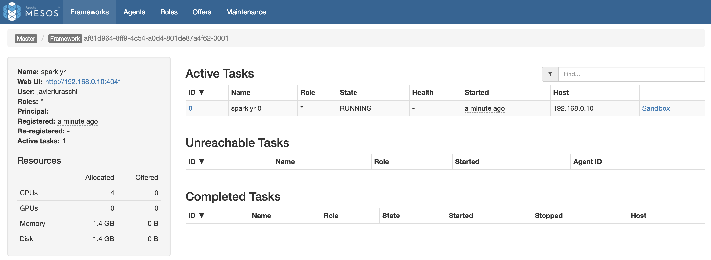 FIGURE 6.6: Mesos web interface running Spark and R
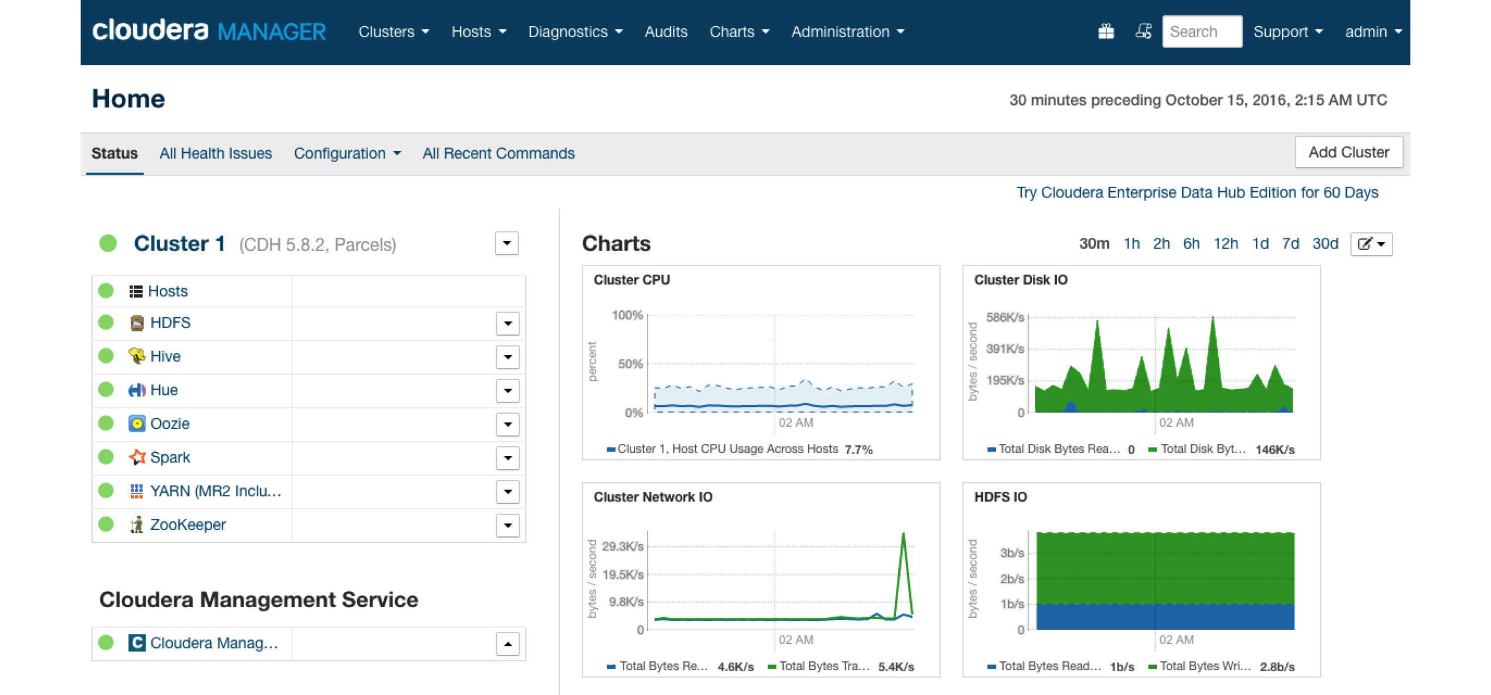 FIGURE 6.7: Cloudera Manager running Spark parcel
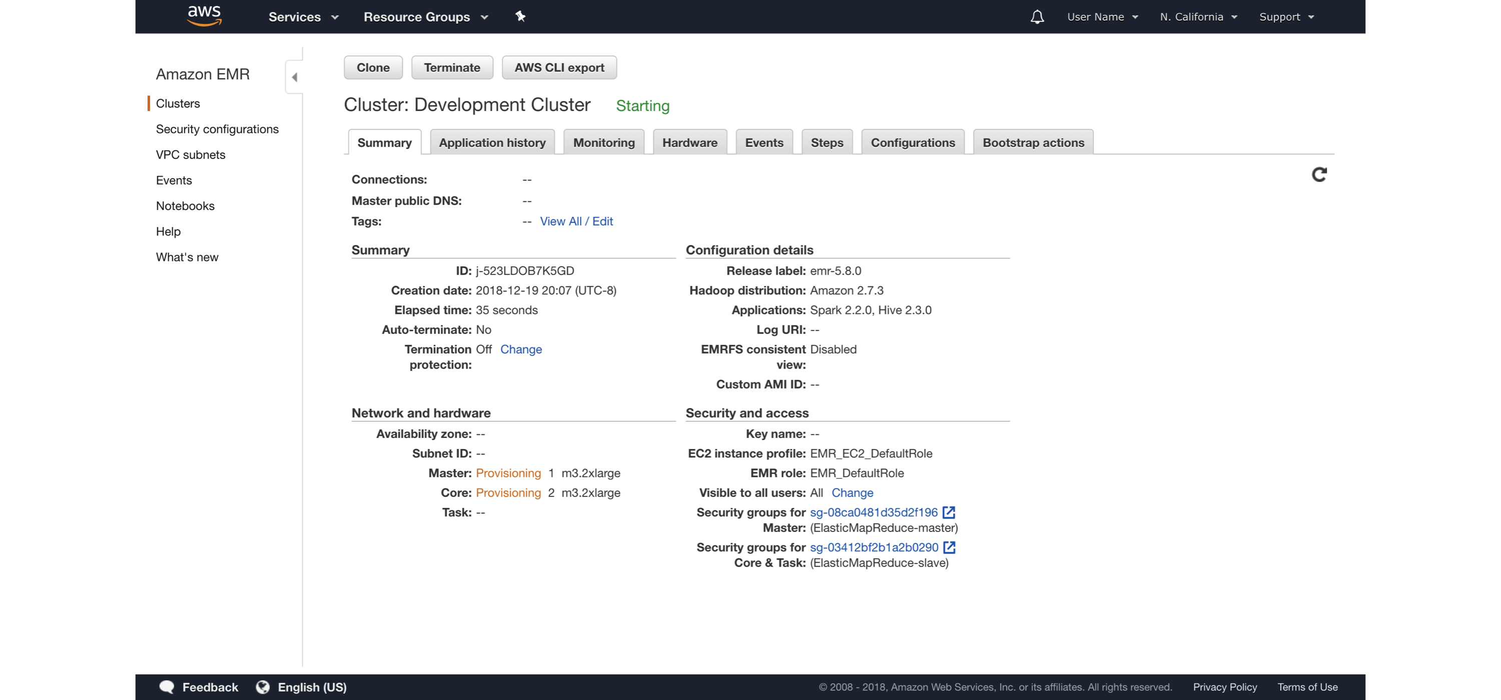 FIGURE 6.8: Launching an Amazon EMR cluster
It is also possible to launch the Amazon EMR cluster using the web interface; the same introductory post contains additional details and walkthroughs specifically designed for Amazon EMR.
Remember to turn off your cluster to avoid unnecessary charges and use appropriate security restrictions when starting Amazon EMR clusters for sensitive data analysis.
Regarding cost, you can find the most up-to-date information at https://amzn.to/2YRGb5r[Amazon EMR Pricing].
Table 6.2 presents some of the instance types available in the
FIGURE 6.8: Launching an Amazon EMR cluster
It is also possible to launch the Amazon EMR cluster using the web interface; the same introductory post contains additional details and walkthroughs specifically designed for Amazon EMR.
Remember to turn off your cluster to avoid unnecessary charges and use appropriate security restrictions when starting Amazon EMR clusters for sensitive data analysis.
Regarding cost, you can find the most up-to-date information at https://amzn.to/2YRGb5r[Amazon EMR Pricing].
Table 6.2 presents some of the instance types available in the 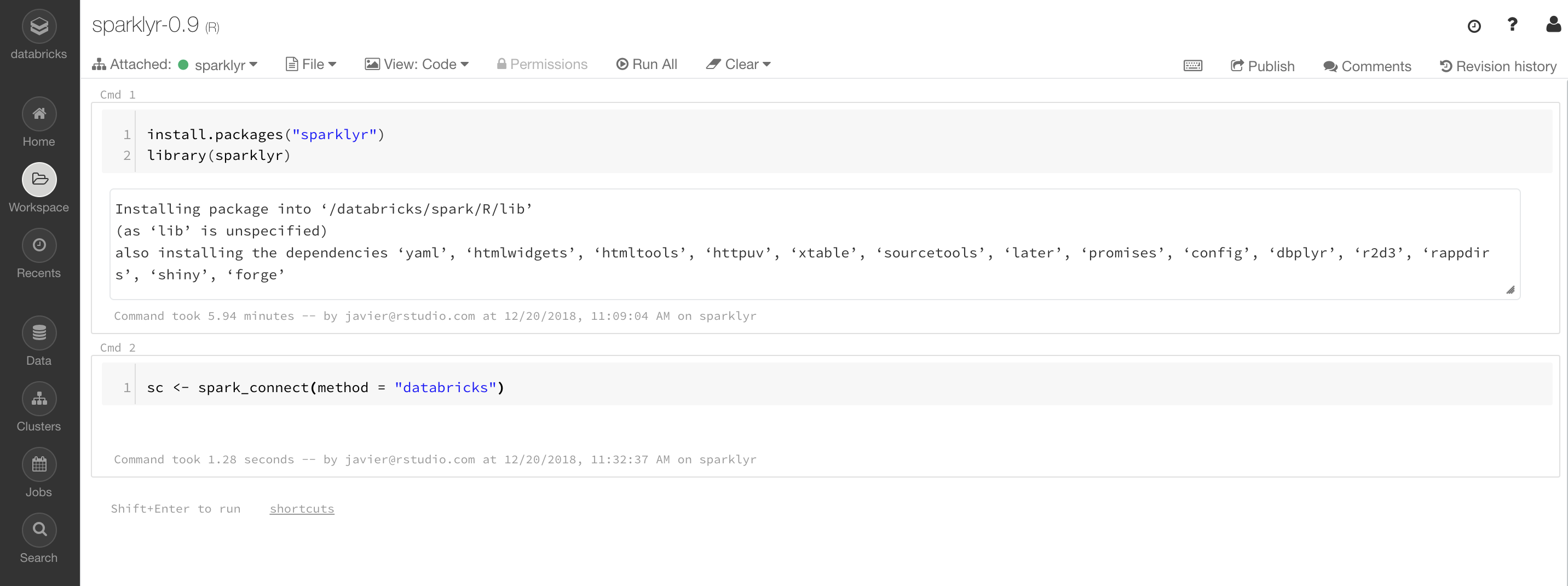 FIGURE 6.9: Databricks community notebook running sparklyr
Additional resources are available under the Databricks Engineering Blog post “Using sparklyr in Databricks” and the Databricks documentation for
FIGURE 6.9: Databricks community notebook running sparklyr
Additional resources are available under the Databricks Engineering Blog post “Using sparklyr in Databricks” and the Databricks documentation for 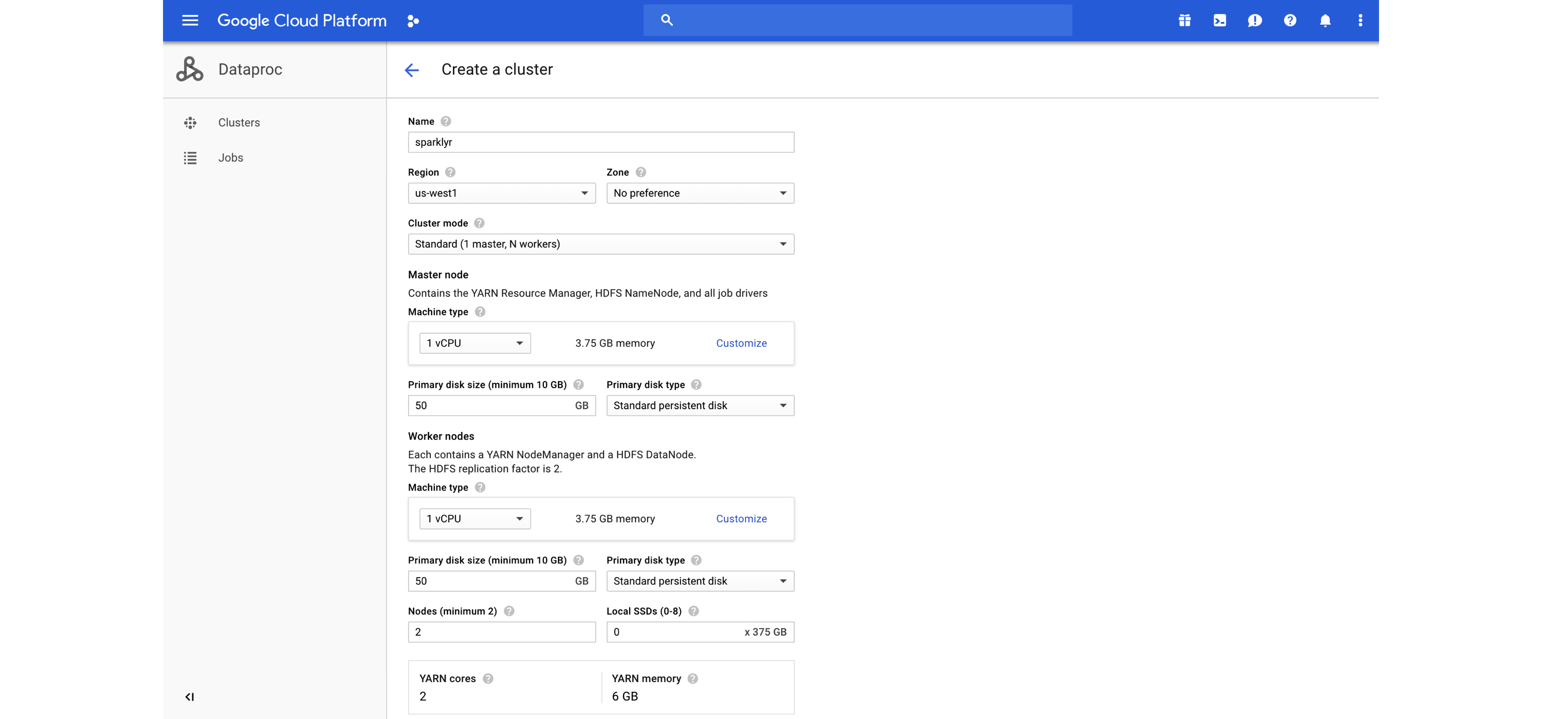 FIGURE 6.10: Launching a Dataproc cluster
After you’ve created your cluster, ports can be forwarded to allow you to access this cluster from your machine—for instance, by launching Chrome to make use of this proxy and securely connect to the Dataproc cluster.
Configuring this connection looks as follows:
FIGURE 6.10: Launching a Dataproc cluster
After you’ve created your cluster, ports can be forwarded to allow you to access this cluster from your machine—for instance, by launching Chrome to make use of this proxy and securely connect to the Dataproc cluster.
Configuring this connection looks as follows:
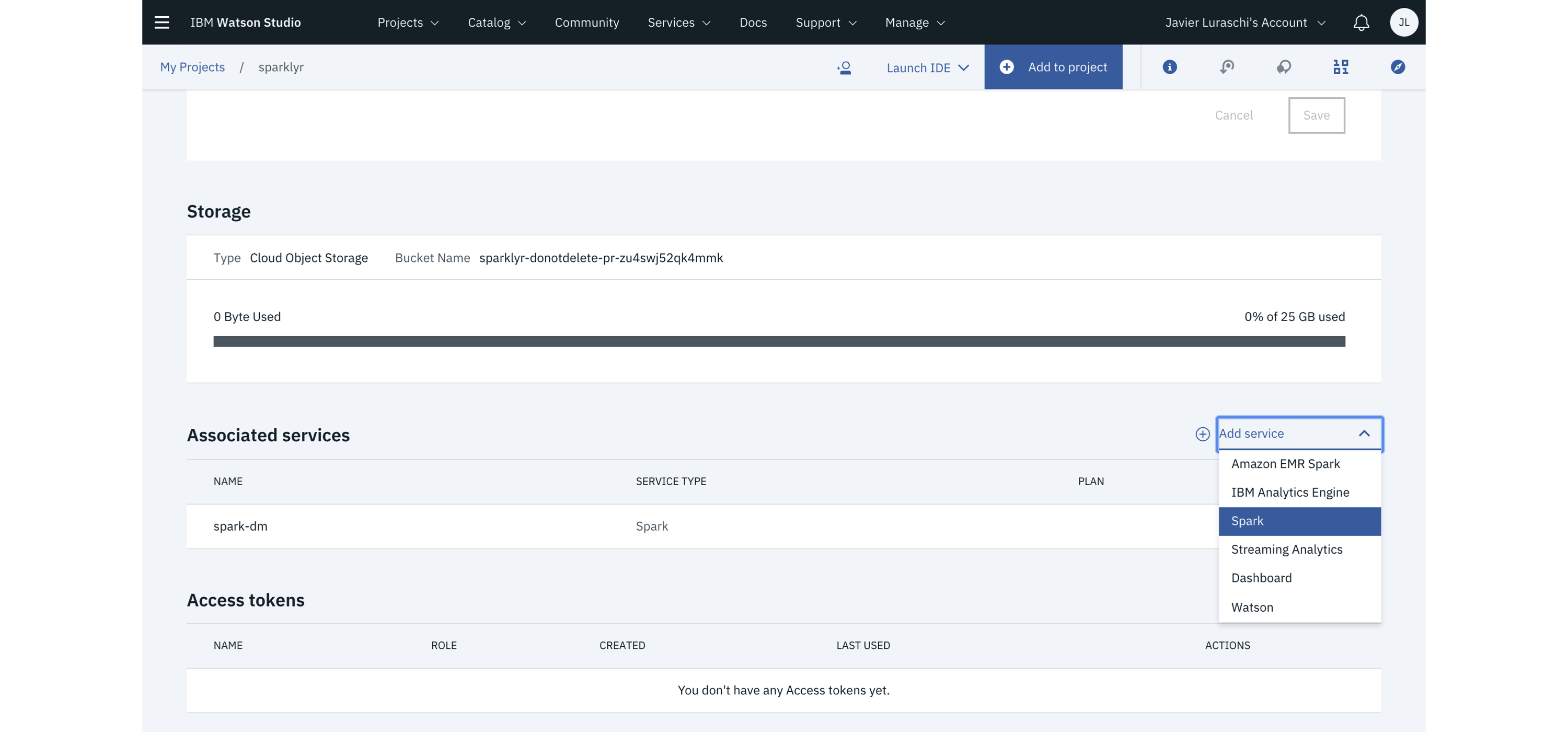 FIGURE 6.11: IBM Watson Studio launching Spark with R support
The most up-to-date pricing information is available at ibm.com/cloud/pricing.
In Table 6.5, compute cost was normalized using 31 days from the per-month costs.
FIGURE 6.11: IBM Watson Studio launching Spark with R support
The most up-to-date pricing information is available at ibm.com/cloud/pricing.
In Table 6.5, compute cost was normalized using 31 days from the per-month costs.
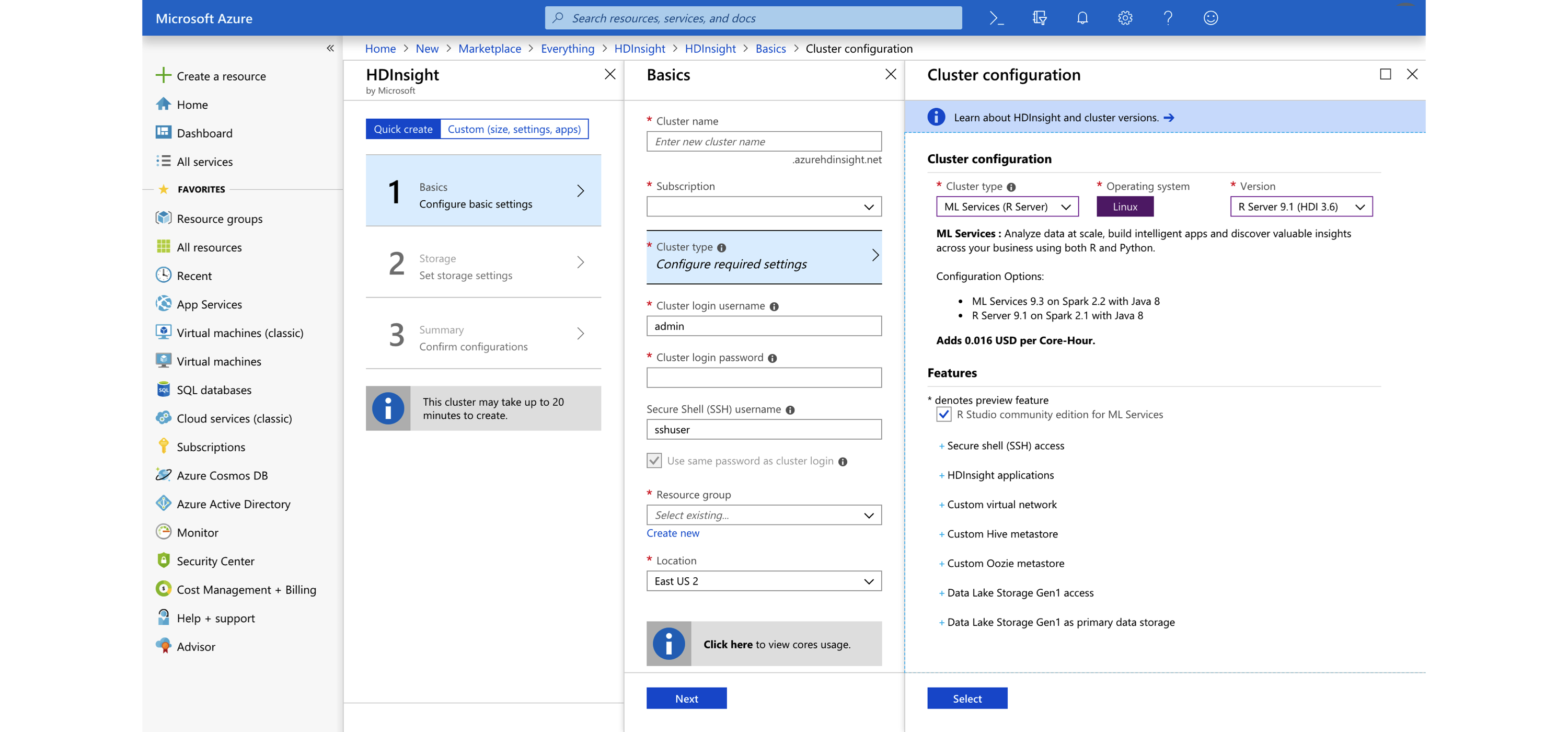 FIGURE 6.12: Creating an Azure HDInsight Spark cluster
Up-to-date pricing for HDInsight is available at azure.microsoft.com/en-us/pricing/details/hdinsight; Table 6.6 lists the pricing as of this writing.
FIGURE 6.12: Creating an Azure HDInsight Spark cluster
Up-to-date pricing for HDInsight is available at azure.microsoft.com/en-us/pricing/details/hdinsight; Table 6.6 lists the pricing as of this writing.
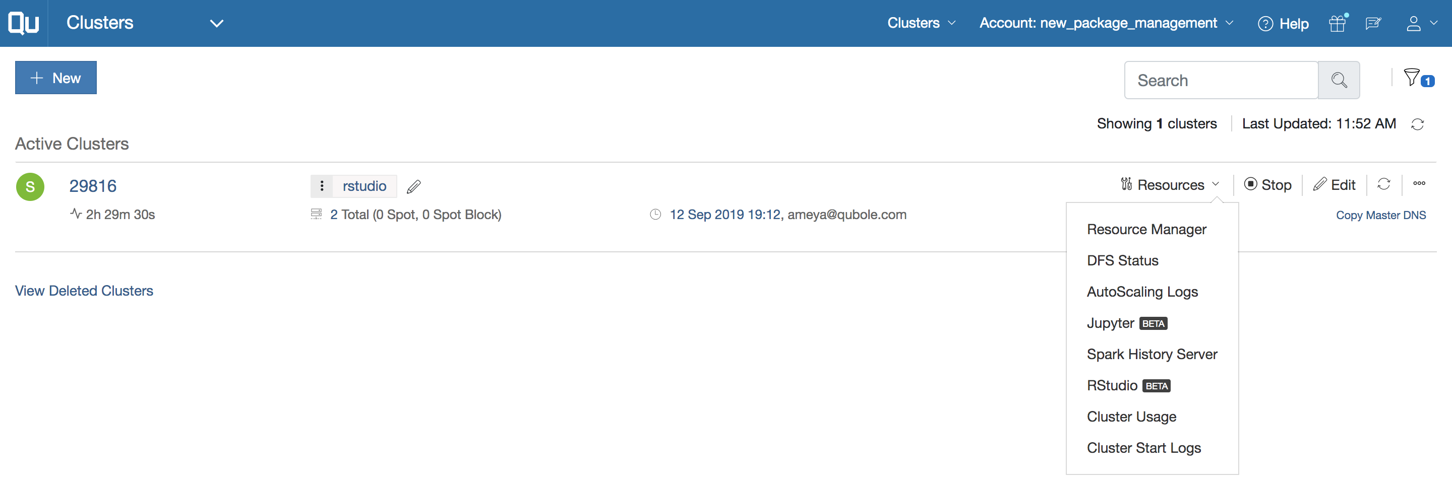 FIGURE 6.13: A Qubole cluster initialized with RStudio and sparklyr
You can find the latest pricing information at http://bit.ly/33AuKh8[Qubole's pricing page].
Table 6.7 lists the price for Qubole’s current plan, as of this writing.
Notice that pricing is based on cost of QCU/hr, which stands for “Qubole Compute Unit per hour,” and the Enterprise Edition requires an annual contract.
FIGURE 6.13: A Qubole cluster initialized with RStudio and sparklyr
You can find the latest pricing information at http://bit.ly/33AuKh8[Qubole's pricing page].
Table 6.7 lists the price for Qubole’s current plan, as of this writing.
Notice that pricing is based on cost of QCU/hr, which stands for “Qubole Compute Unit per hour,” and the Enterprise Edition requires an annual contract.
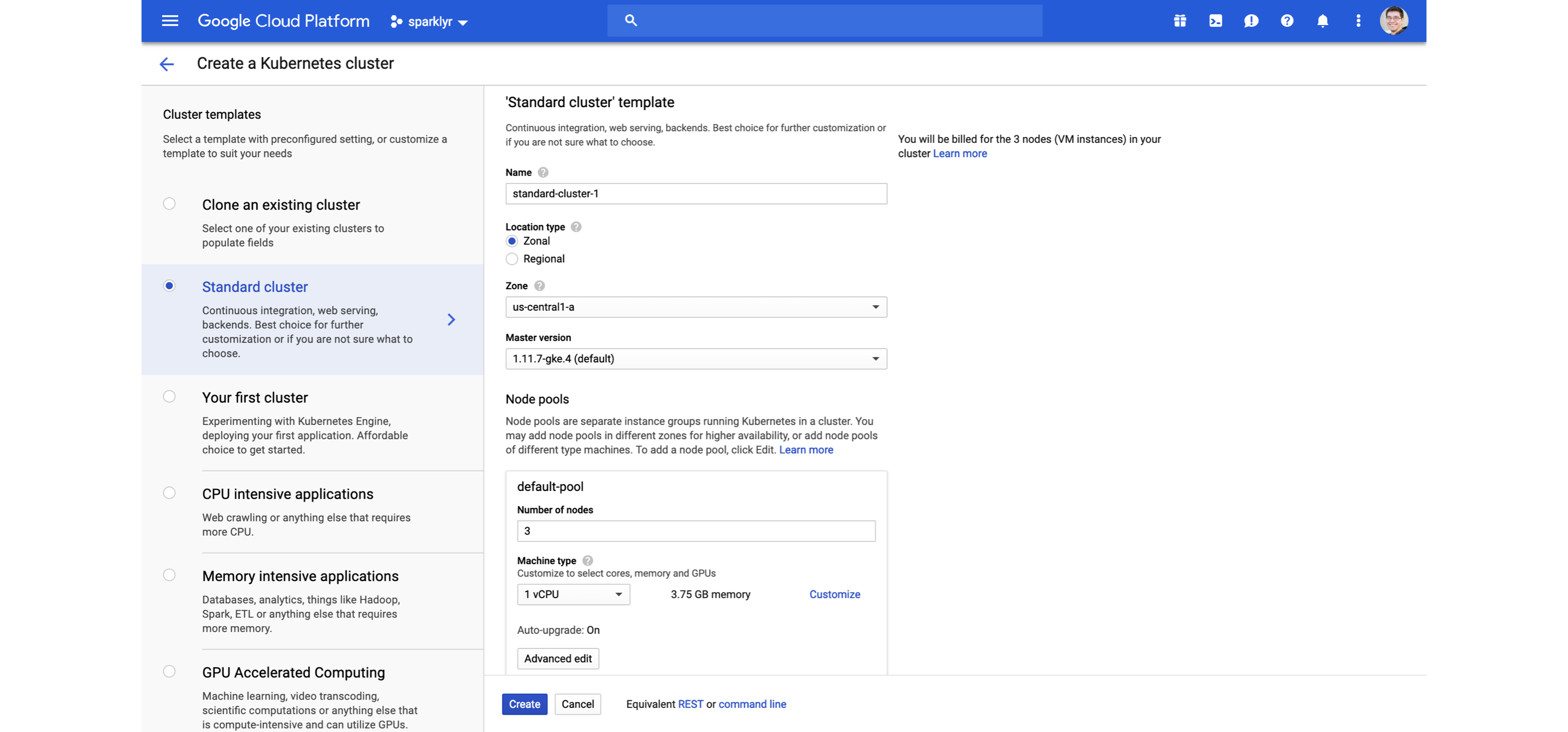 FIGURE 6.14: Creating a Kubernetes cluster for Spark and R using Google Cloud
You can learn more at kubernetes.io, and read the Running Spark on Kubernetes guide from spark.apache.org.
Strictly speaking, Kubernetes is a cluster technology, not a specific cluster architecture.
However, Kubernetes represents a larger trend often referred to as a hybrid cloud.
A hybrid cloud is a computing environment that makes use of on-premises and public cloud services with orchestration between the various platforms.
It’s still too early to precisely categorize the leading technologies that will form a hybrid approach to cluster computing; although, as previously mentioned, Kubernetes is the leading one, many more are likely to form to complement or even replace existing technologies.
FIGURE 6.14: Creating a Kubernetes cluster for Spark and R using Google Cloud
You can learn more at kubernetes.io, and read the Running Spark on Kubernetes guide from spark.apache.org.
Strictly speaking, Kubernetes is a cluster technology, not a specific cluster architecture.
However, Kubernetes represents a larger trend often referred to as a hybrid cloud.
A hybrid cloud is a computing environment that makes use of on-premises and public cloud services with orchestration between the various platforms.
It’s still too early to precisely categorize the leading technologies that will form a hybrid approach to cluster computing; although, as previously mentioned, Kubernetes is the leading one, many more are likely to form to complement or even replace existing technologies.
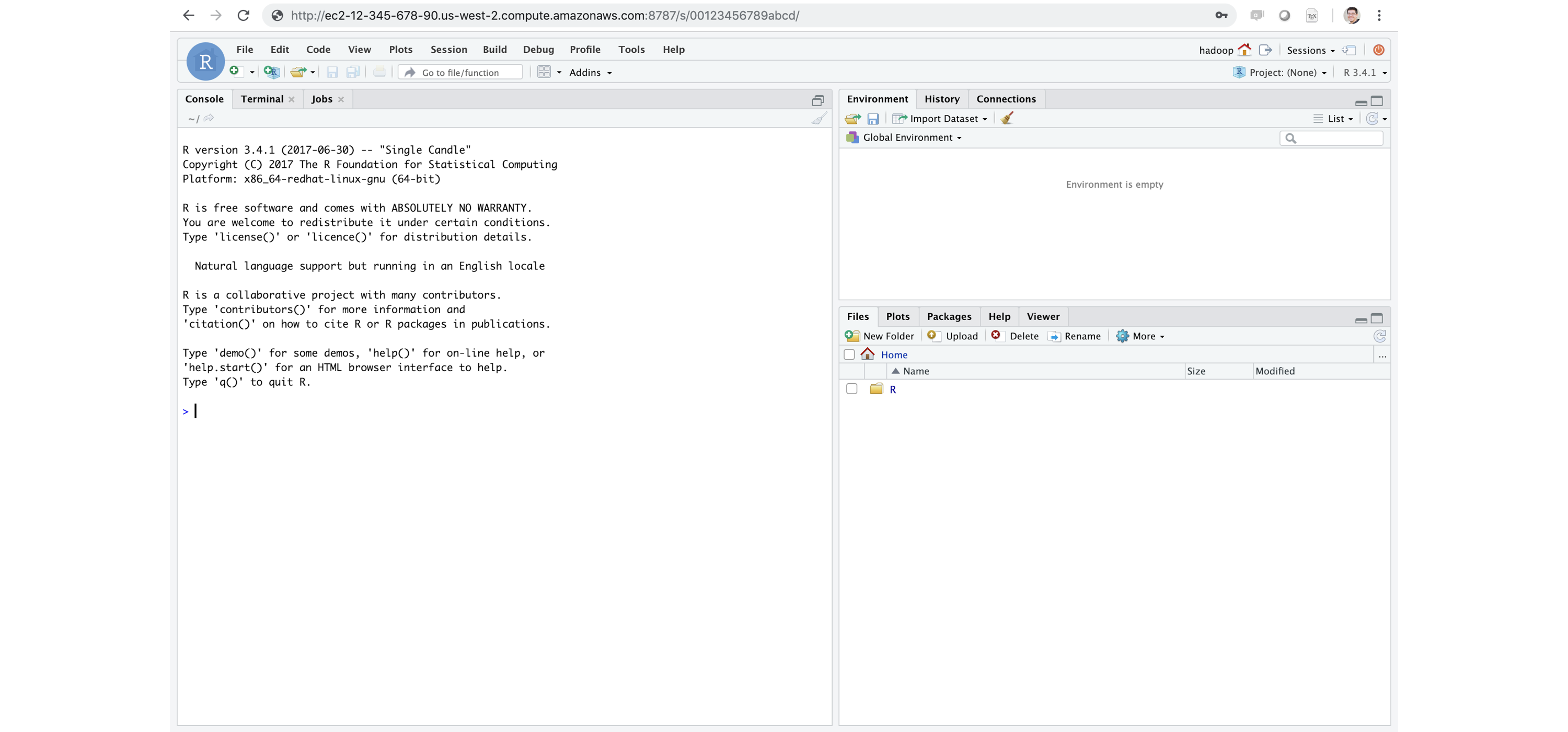 FIGURE 6.15: RStudio Server Pro running inside Apache Spark
If you’re familiar with R, Shiny Server is a very popular tool for building interactive web applications from R.
We recommended that you install Shiny directly in your Spark cluster.
RStudio Server and Shiny Server are a free and open source; however, RStudio also provides professional products like RStudio Server, RStudio Server Pro, Shiny Server Pro, and RStudio Connect, which you can install within the cluster to support additional R workflows.
While
FIGURE 6.15: RStudio Server Pro running inside Apache Spark
If you’re familiar with R, Shiny Server is a very popular tool for building interactive web applications from R.
We recommended that you install Shiny directly in your Spark cluster.
RStudio Server and Shiny Server are a free and open source; however, RStudio also provides professional products like RStudio Server, RStudio Server Pro, Shiny Server Pro, and RStudio Connect, which you can install within the cluster to support additional R workflows.
While 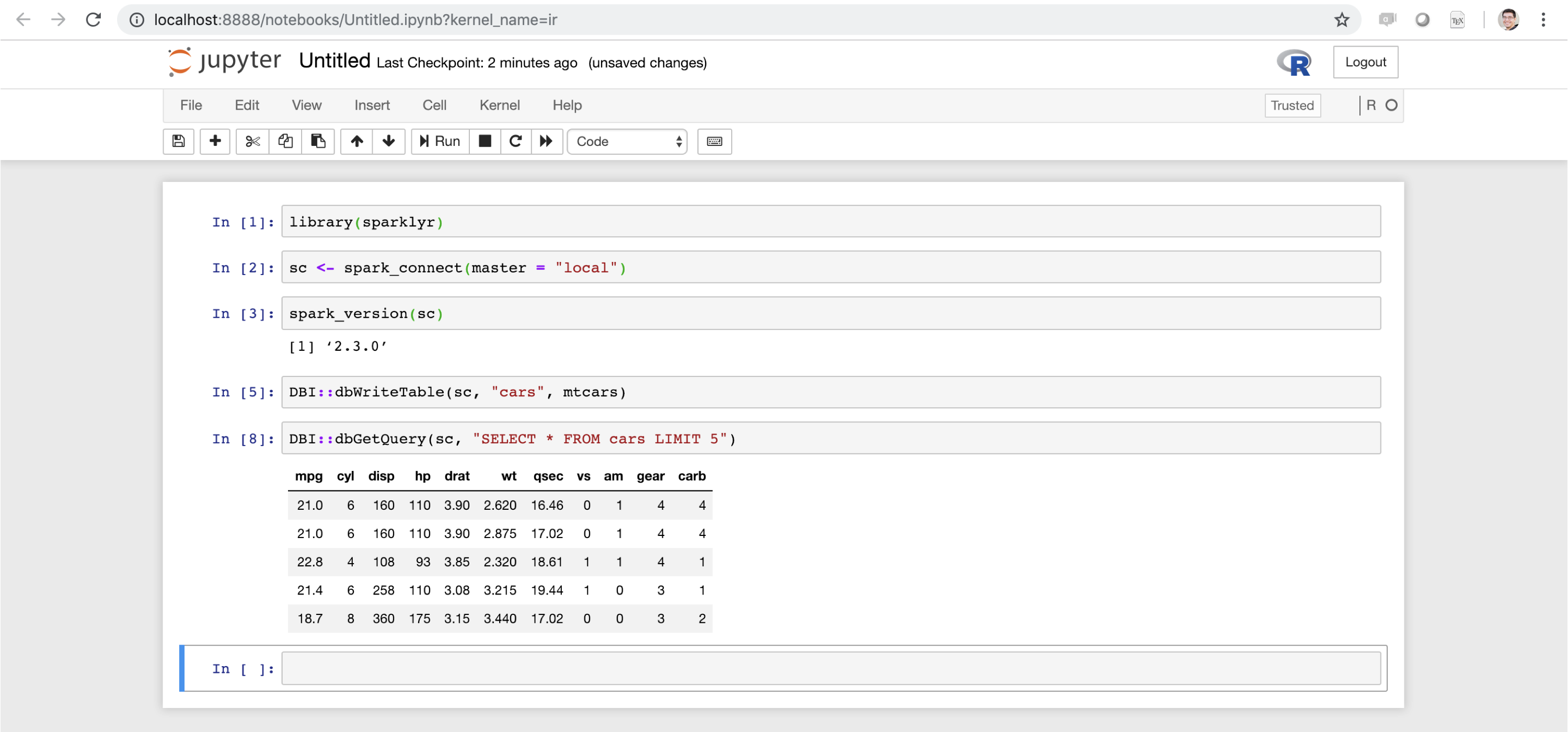 FIGURE 6.16: Jupyter notebook running sparklyr
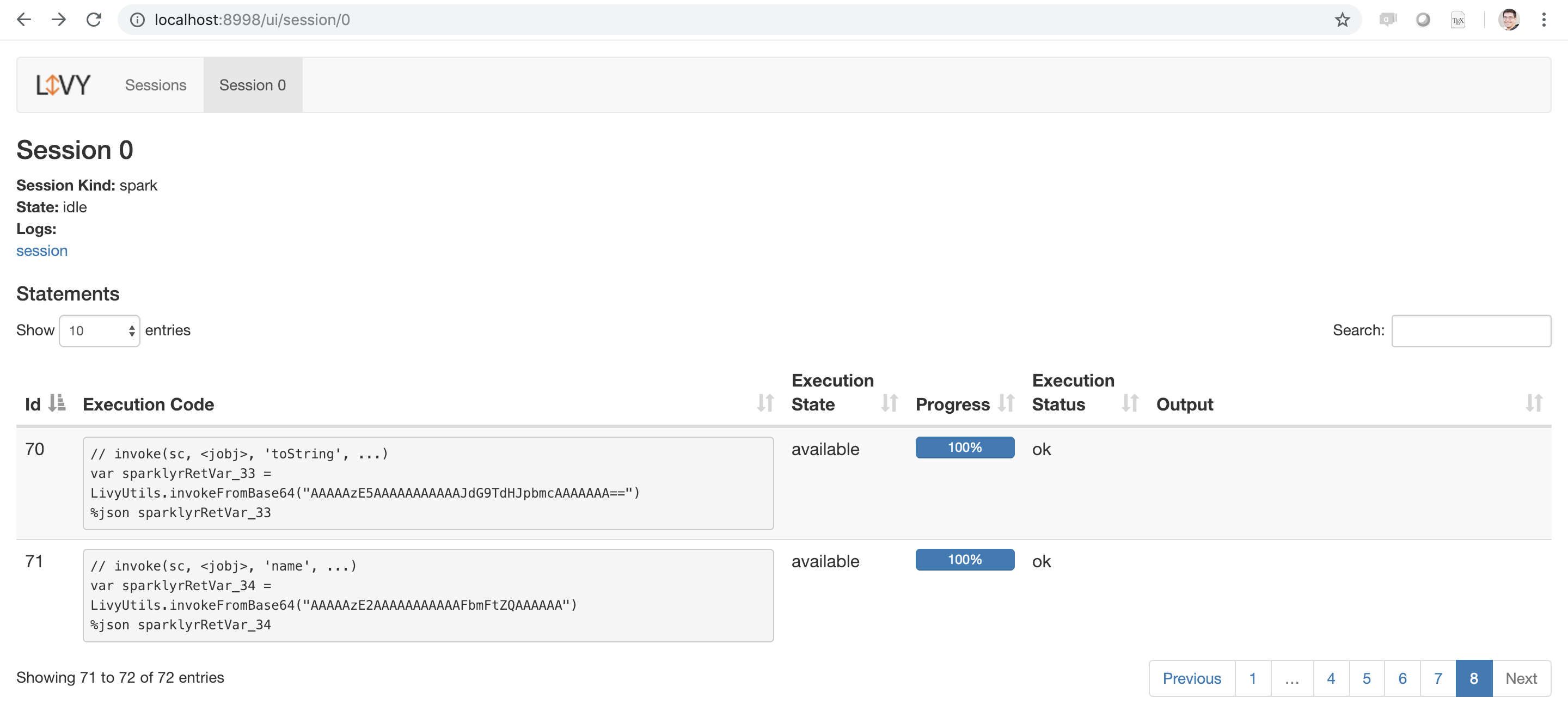 FIGURE 6.17: Apache Livy running as a local service
Make sure you also stop the Livy service when working with local Livy instances (for proper Livy services running in a cluster, you won’t have to):
FIGURE 6.17: Apache Livy running as a local service
Make sure you also stop the Livy service when working with local Livy instances (for proper Livy services running in a cluster, you won’t have to):
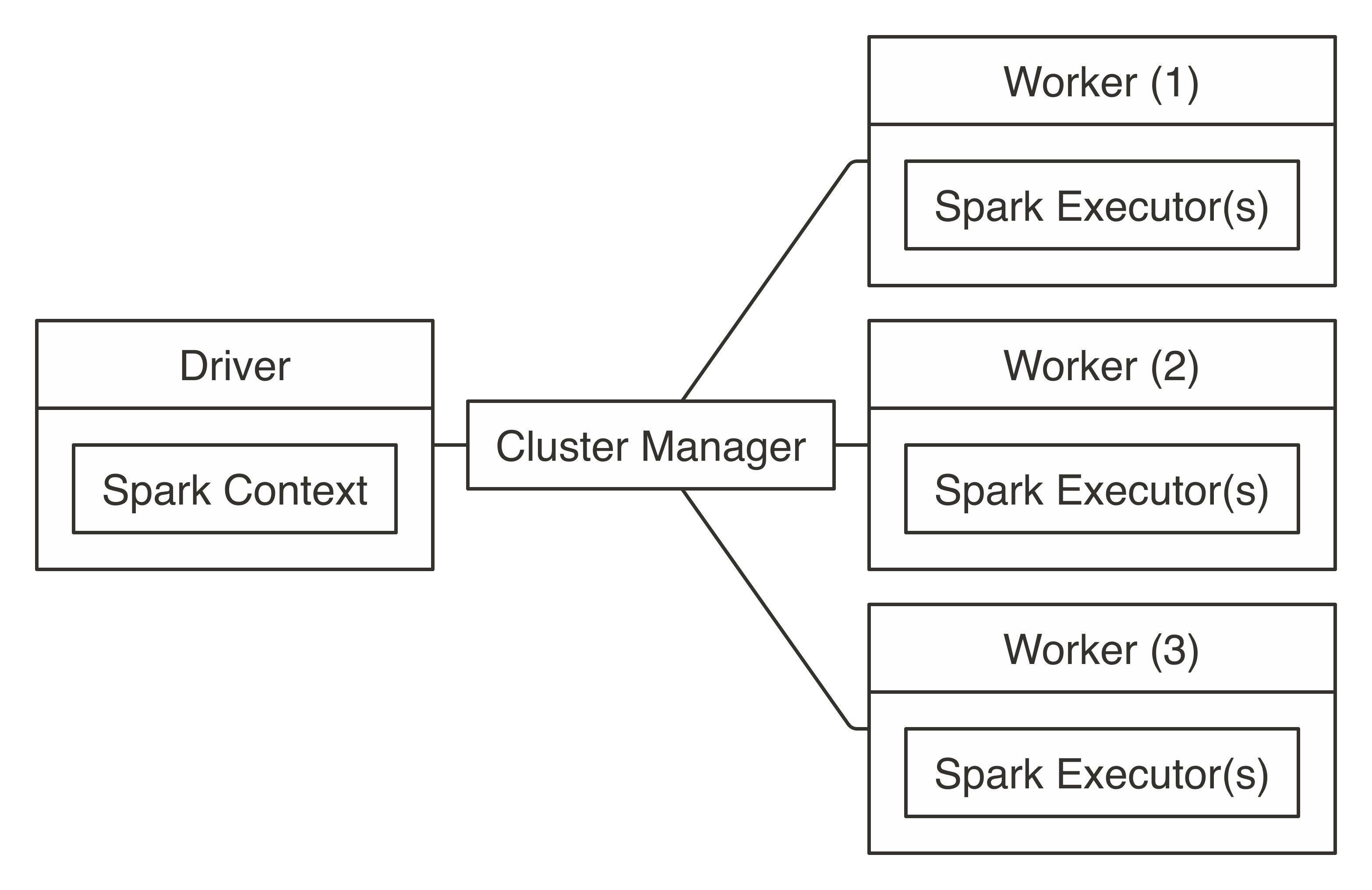 FIGURE 7.1: Apache Spark connection architecture
If you already have a Spark cluster in your organization, you should request the connection information to this cluster from your cluster administrator, read their usage policies carefully, and follow their advice.
Since a cluster can be shared among many users, you want to ensure that you request only the compute resources you need.
We cover how to request resources in Chapter 9.
Your system administrator will specify whether it’s an on-premises or cloud cluster, the cluster manager being used, supported connections, and supported tools.
You can use this information to jump directly to Standalone, YARN, Mesos, Livy, or Kubernetes based on which is appropriate for your situation.
Note: After you’ve used
FIGURE 7.1: Apache Spark connection architecture
If you already have a Spark cluster in your organization, you should request the connection information to this cluster from your cluster administrator, read their usage policies carefully, and follow their advice.
Since a cluster can be shared among many users, you want to ensure that you request only the compute resources you need.
We cover how to request resources in Chapter 9.
Your system administrator will specify whether it’s an on-premises or cloud cluster, the cluster manager being used, supported connections, and supported tools.
You can use this information to jump directly to Standalone, YARN, Mesos, Livy, or Kubernetes based on which is appropriate for your situation.
Note: After you’ve used  FIGURE 7.2: Connecting to Spark’s edge node
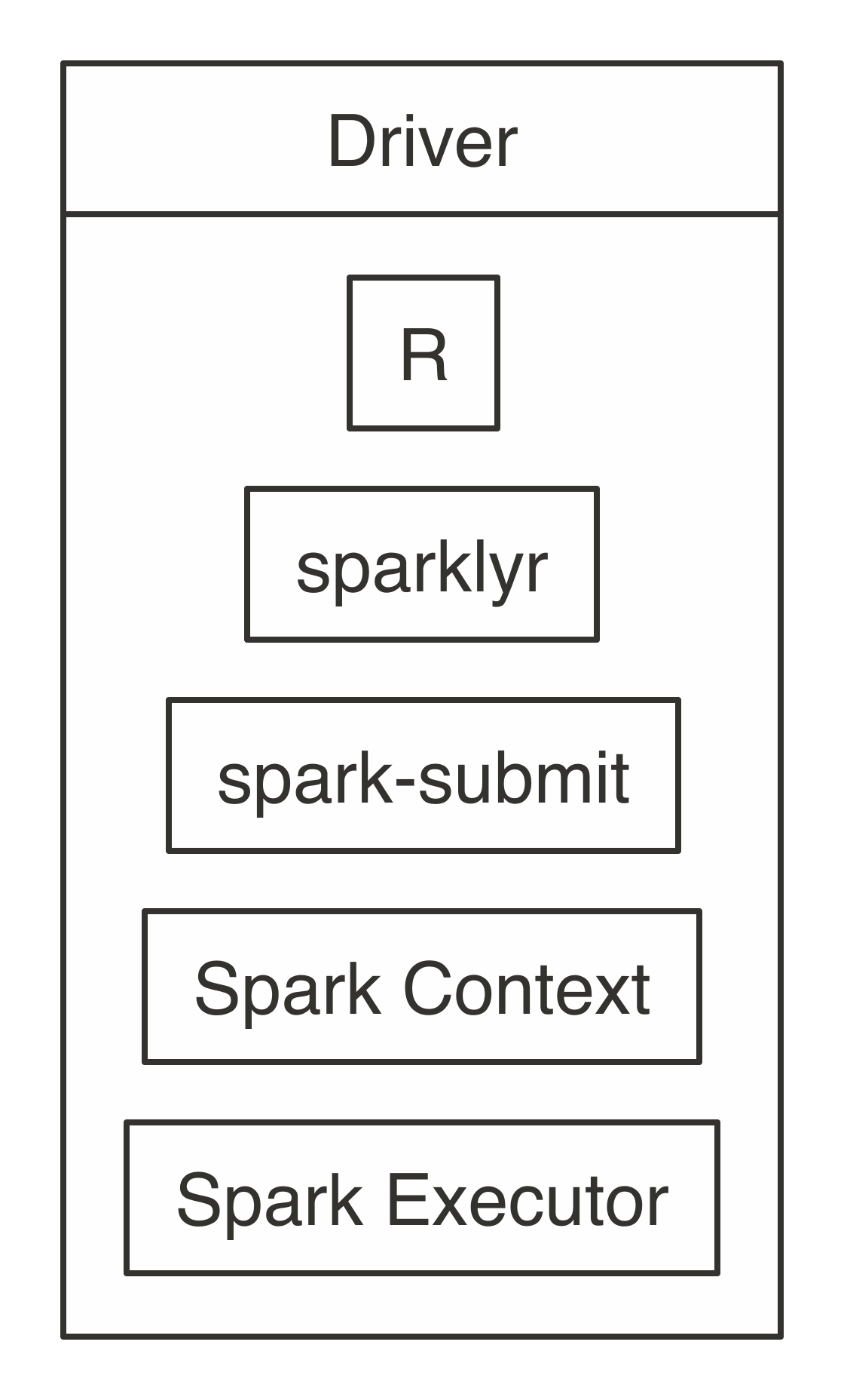 FIGURE 7.3: Local connection diagram
Notice that there is neither a cluster manager nor worker process since, in local mode, everything runs inside the driver application.
It’s also worth noting that
FIGURE 7.3: Local connection diagram
Notice that there is neither a cluster manager nor worker process since, in local mode, everything runs inside the driver application.
It’s also worth noting that 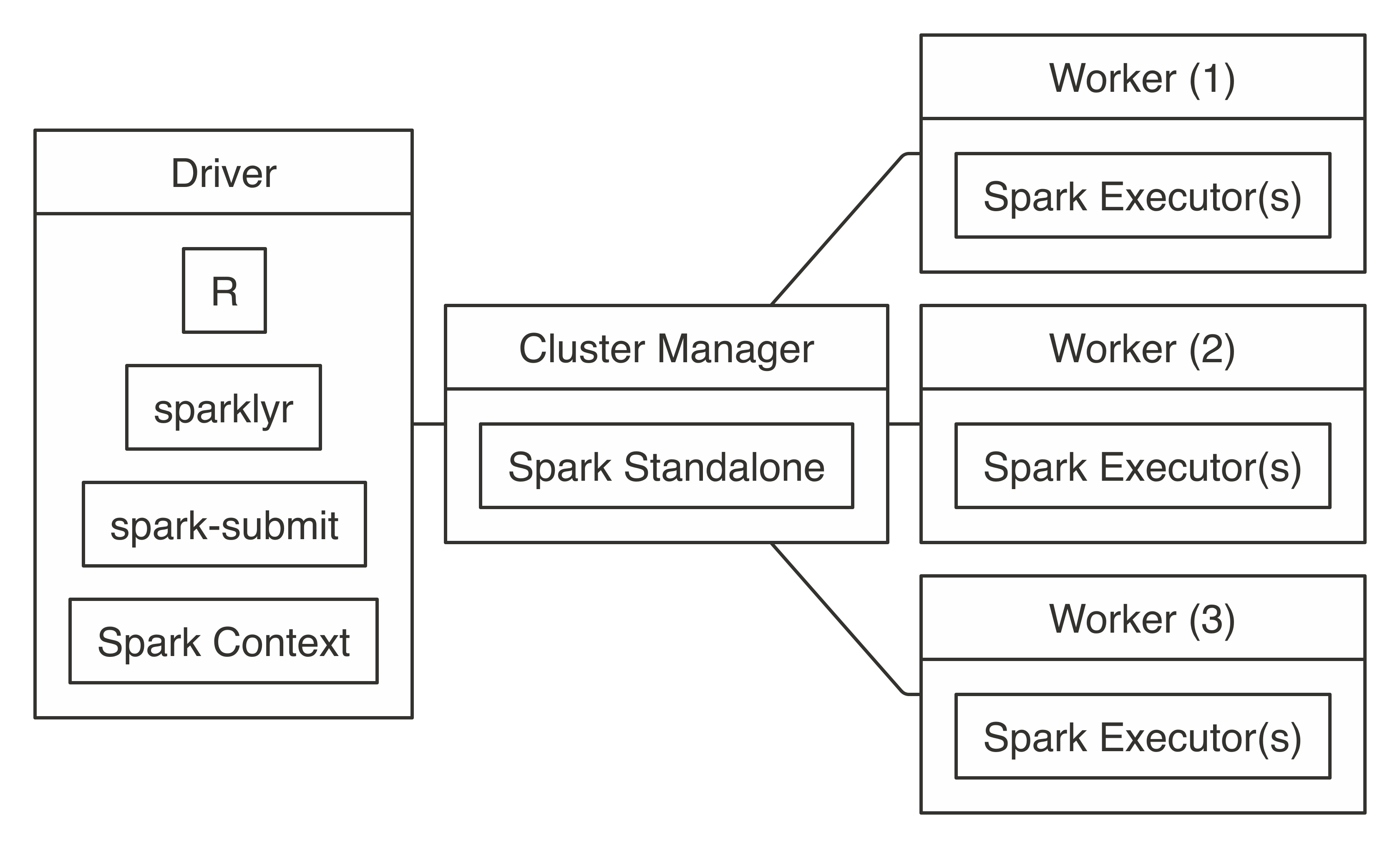 FIGURE 7.4: Spark Standalone connection diagram
To connect, use
FIGURE 7.4: Spark Standalone connection diagram
To connect, use 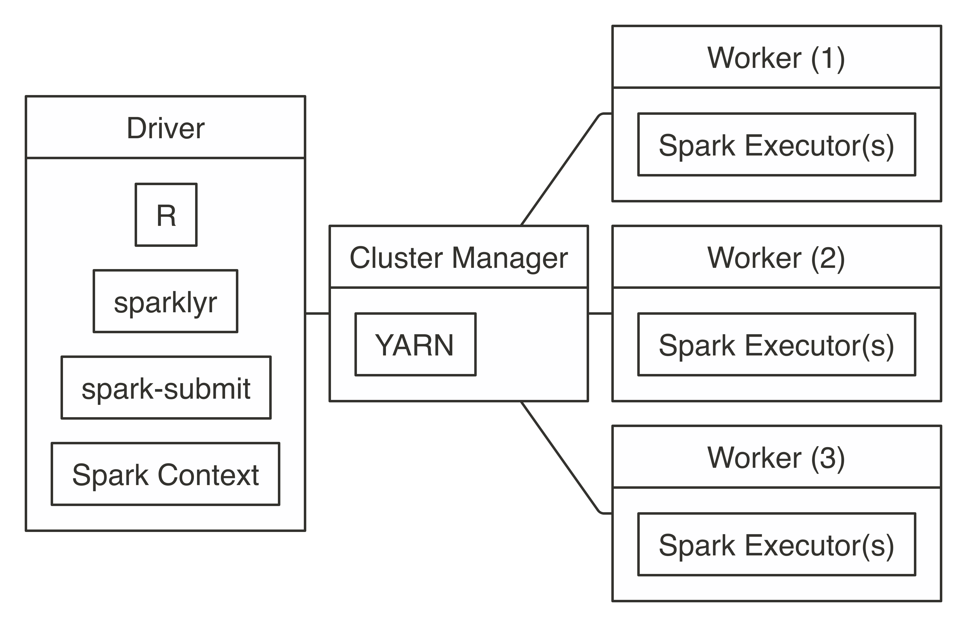 FIGURE 7.5: YARN client connection diagram
To connect, you simply run with
FIGURE 7.5: YARN client connection diagram
To connect, you simply run with 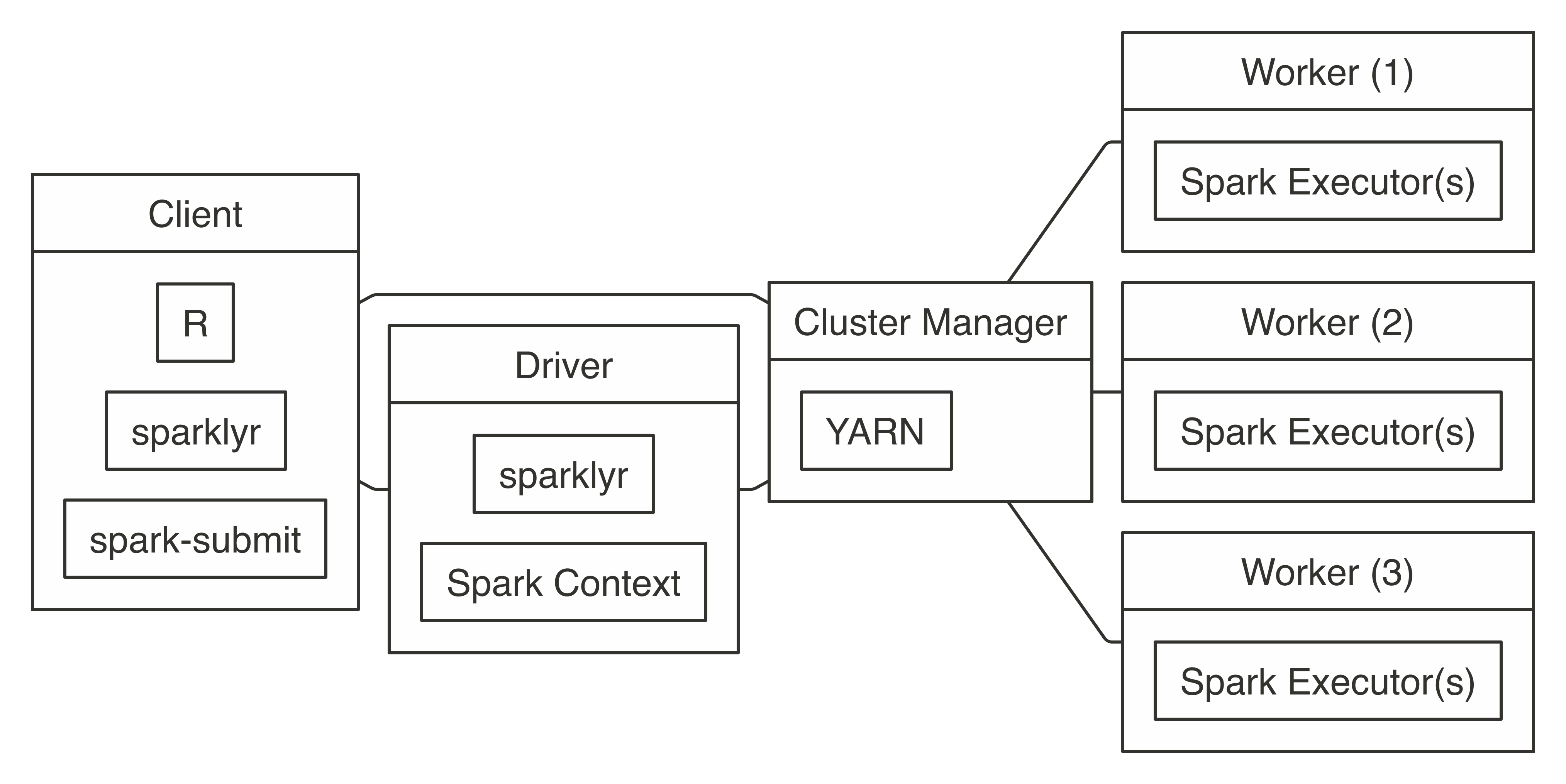 FIGURE 7.6: YARN cluster connection diagram
To connect in YARN cluster mode, simply run the following:
FIGURE 7.6: YARN cluster connection diagram
To connect in YARN cluster mode, simply run the following:
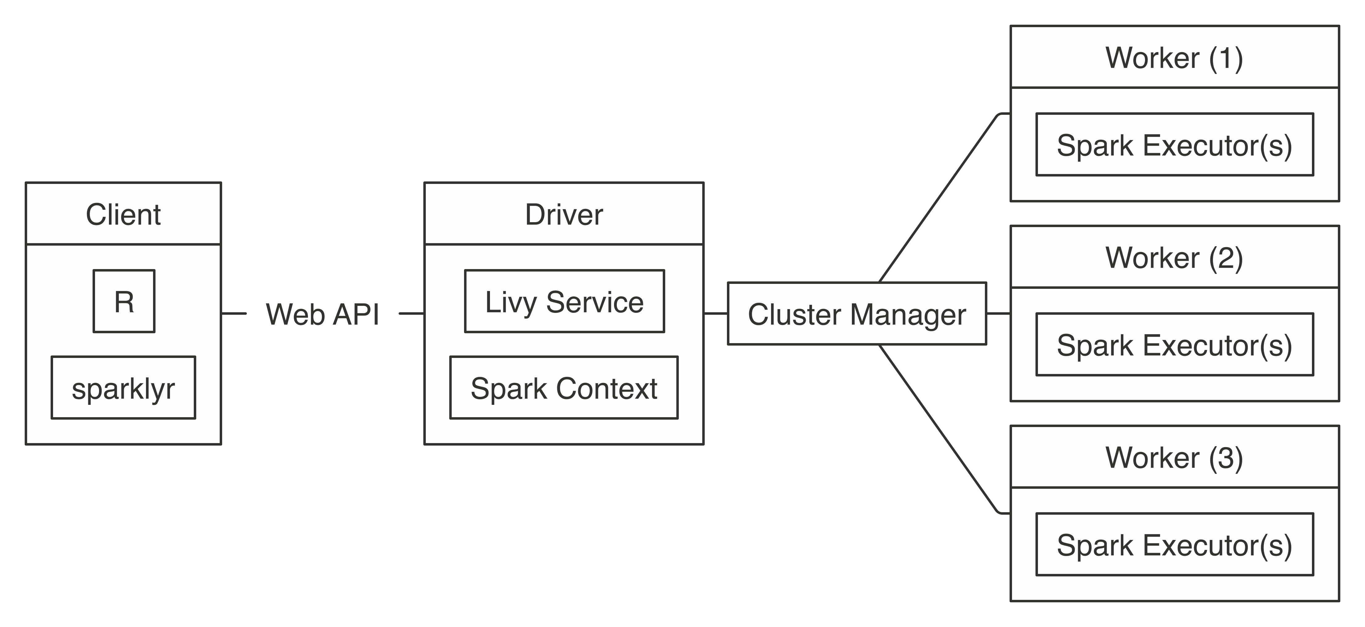 FIGURE 7.7: Livy connection diagram
Connecting through Livy requires the URL to the Livy service, which should be similar to
FIGURE 7.7: Livy connection diagram
Connecting through Livy requires the URL to the Livy service, which should be similar to 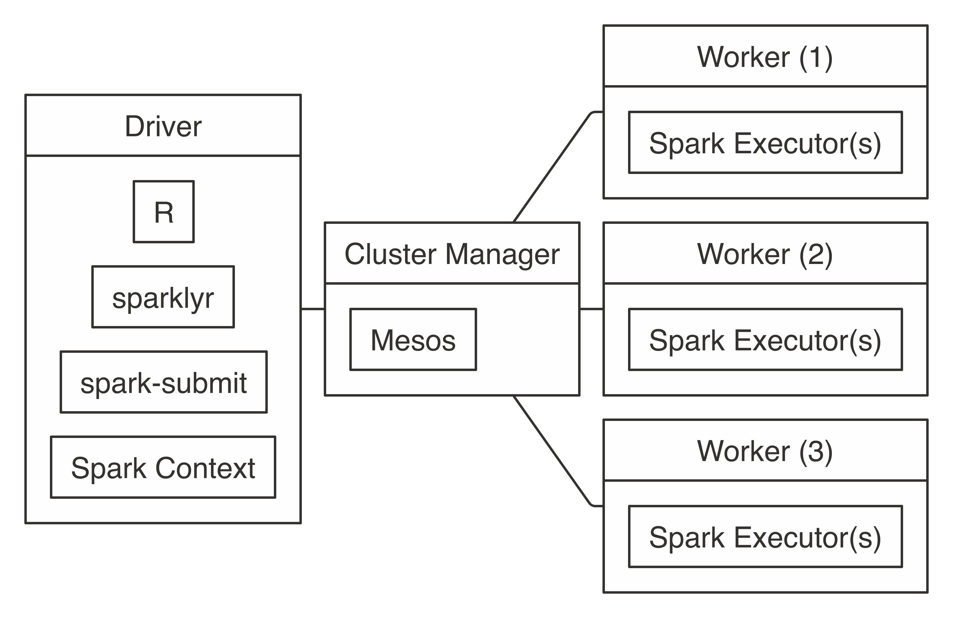 FIGURE 7.8: Mesos connection diagram
Connecting requires the address to the Mesos master node, usually in the form of
FIGURE 7.8: Mesos connection diagram
Connecting requires the address to the Mesos master node, usually in the form of 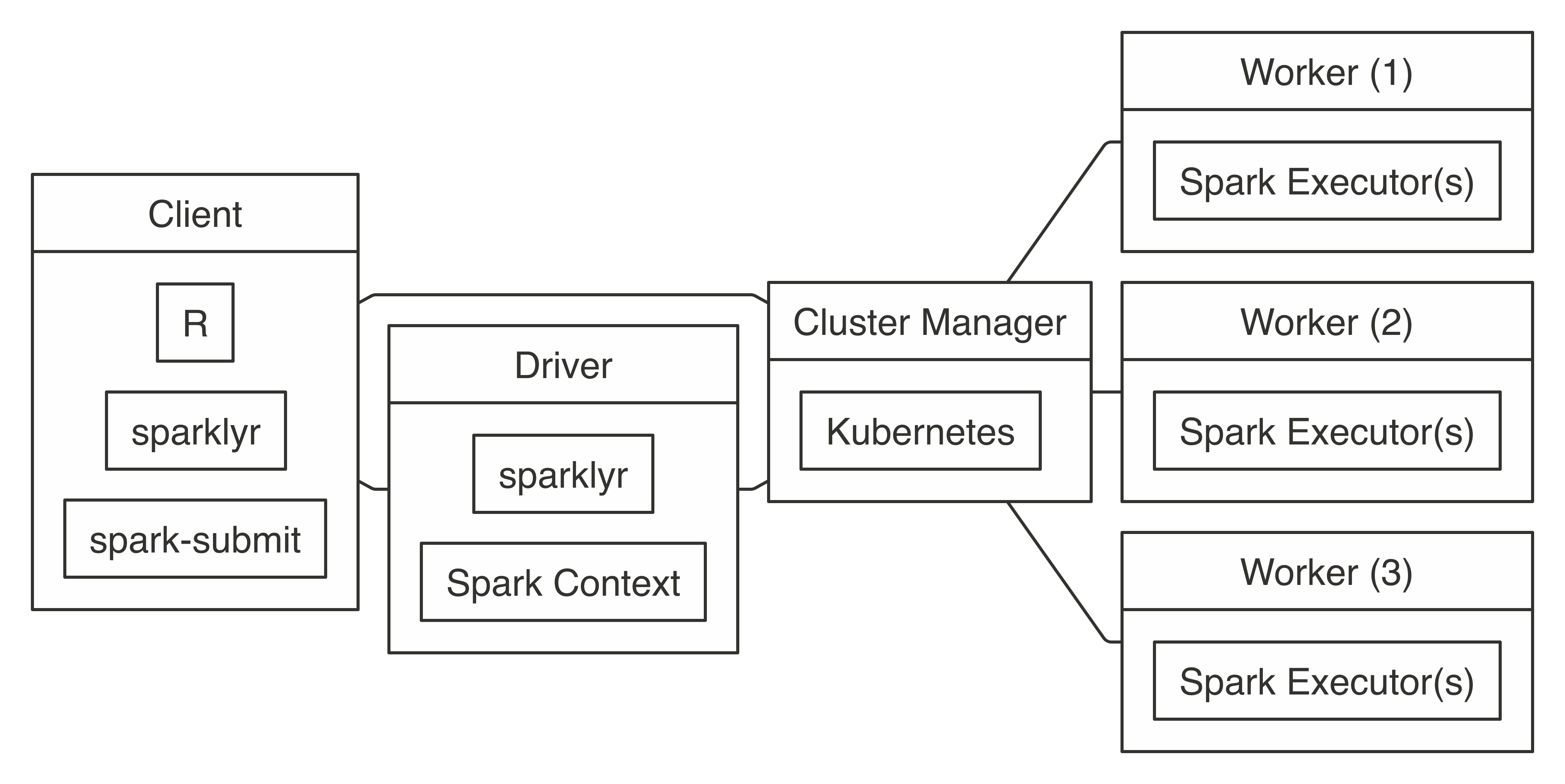 FIGURE 7.9: Kubernetes connection diagram
To use Kubernetes, you will need to prepare a virtual machine with Spark installed and properly configured; however, it is beyond the scope of this book to present how to create one.
Once created, connecting to Kubernetes works as follows:
FIGURE 7.9: Kubernetes connection diagram
To use Kubernetes, you will need to prepare a virtual machine with Spark installed and properly configured; however, it is beyond the scope of this book to present how to create one.
Once created, connecting to Kubernetes works as follows:
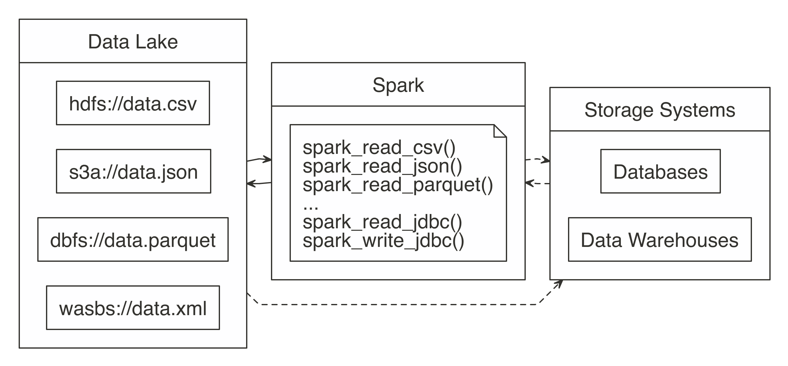 FIGURE 8.1: Spark processing raw data from a data lakes, databases, and data warehouses
In order to support a broad variety of data source, Spark needs to be able to read and write data in several different file formats (CSV, JSON, Parquet, etc), access them while stored in several file systems (HDFS, S3, DBFS, etc) and, potentially, interoperate with other storage systems (databases, data warehouses, etc).
We will get to all of that; but first, we will start by presenting how to read, write and copy data using Spark.
FIGURE 8.1: Spark processing raw data from a data lakes, databases, and data warehouses
In order to support a broad variety of data source, Spark needs to be able to read and write data in several different file formats (CSV, JSON, Parquet, etc), access them while stored in several file systems (HDFS, S3, DBFS, etc) and, potentially, interoperate with other storage systems (databases, data warehouses, etc).
We will get to all of that; but first, we will start by presenting how to read, write and copy data using Spark.
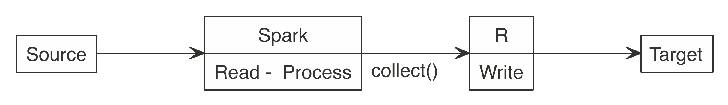 FIGURE 8.2: Incorrect use of Spark when writing large datasets
All efforts should be made to have Spark connect to the target location.
This way, reading, processing, and writing happens within the same Spark session.
As Figure 8.3 shows, a better approach is to use Spark to read, process, and write to the target.
This approach is able to scale as big as the Spark cluster allows, and prevents R from becoming a choke point.
FIGURE 8.2: Incorrect use of Spark when writing large datasets
All efforts should be made to have Spark connect to the target location.
This way, reading, processing, and writing happens within the same Spark session.
As Figure 8.3 shows, a better approach is to use Spark to read, process, and write to the target.
This approach is able to scale as big as the Spark cluster allows, and prevents R from becoming a choke point.
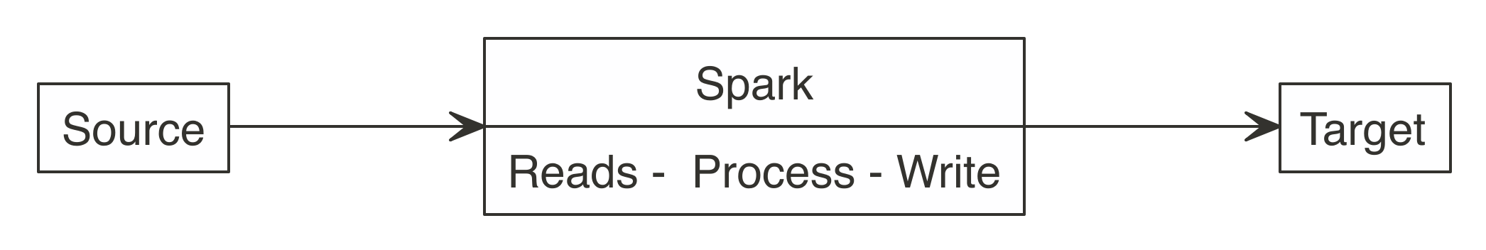 FIGURE 8.3: Correct use of Spark when writing large datasets
Consider the following scenario: a Spark job just processed predictions for a large dataset, resulting in a considerable amount of predictions.
Choosing a method to write results will depend on the technology infrastructure you are working on.
More specifically, it will depend on Spark and the target running, or not, in the same cluster.
Back to our scenario, we have a large dataset in Spark that needs to be saved.
When Spark and the target are in the same cluster, copying the results is not a problem; the data transfer is between RAM and disk of the same cluster or efficiently shuffled through a high-bandwidth connection.
But what to do if the target is not within the Spark cluster? There are two options, and choosing one will depend on the size of the data and network speed:
FIGURE 8.3: Correct use of Spark when writing large datasets
Consider the following scenario: a Spark job just processed predictions for a large dataset, resulting in a considerable amount of predictions.
Choosing a method to write results will depend on the technology infrastructure you are working on.
More specifically, it will depend on Spark and the target running, or not, in the same cluster.
Back to our scenario, we have a large dataset in Spark that needs to be saved.
When Spark and the target are in the same cluster, copying the results is not a problem; the data transfer is between RAM and disk of the same cluster or efficiently shuffled through a high-bandwidth connection.
But what to do if the target is not within the Spark cluster? There are two options, and choosing one will depend on the size of the data and network speed:
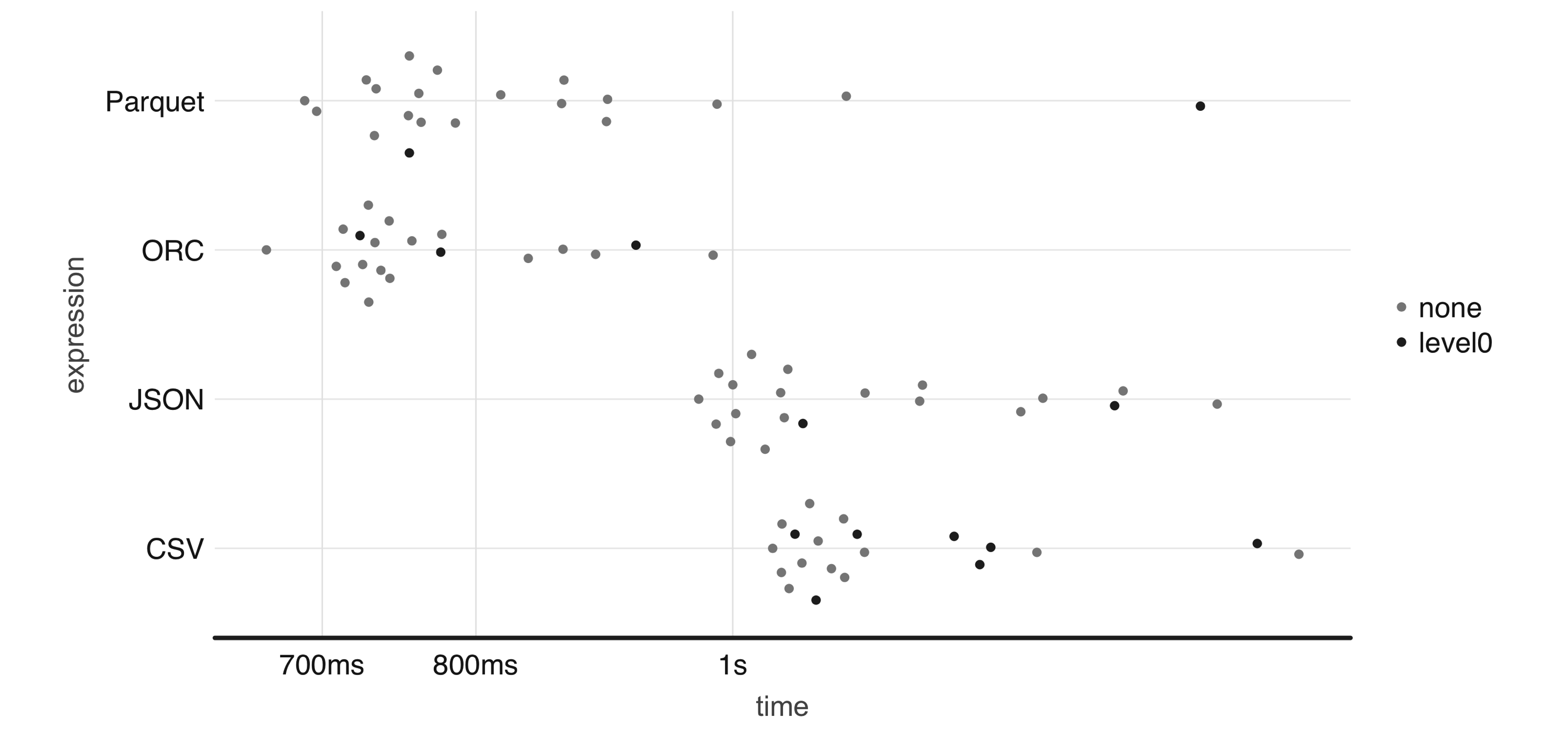 FIGURE 8.4: One-million-rows write benchmark between CSV, JSON, Parquet, and ORC
From now on, be sure to disconnect from Spark whenever we present a new
FIGURE 8.4: One-million-rows write benchmark between CSV, JSON, Parquet, and ORC
From now on, be sure to disconnect from Spark whenever we present a new 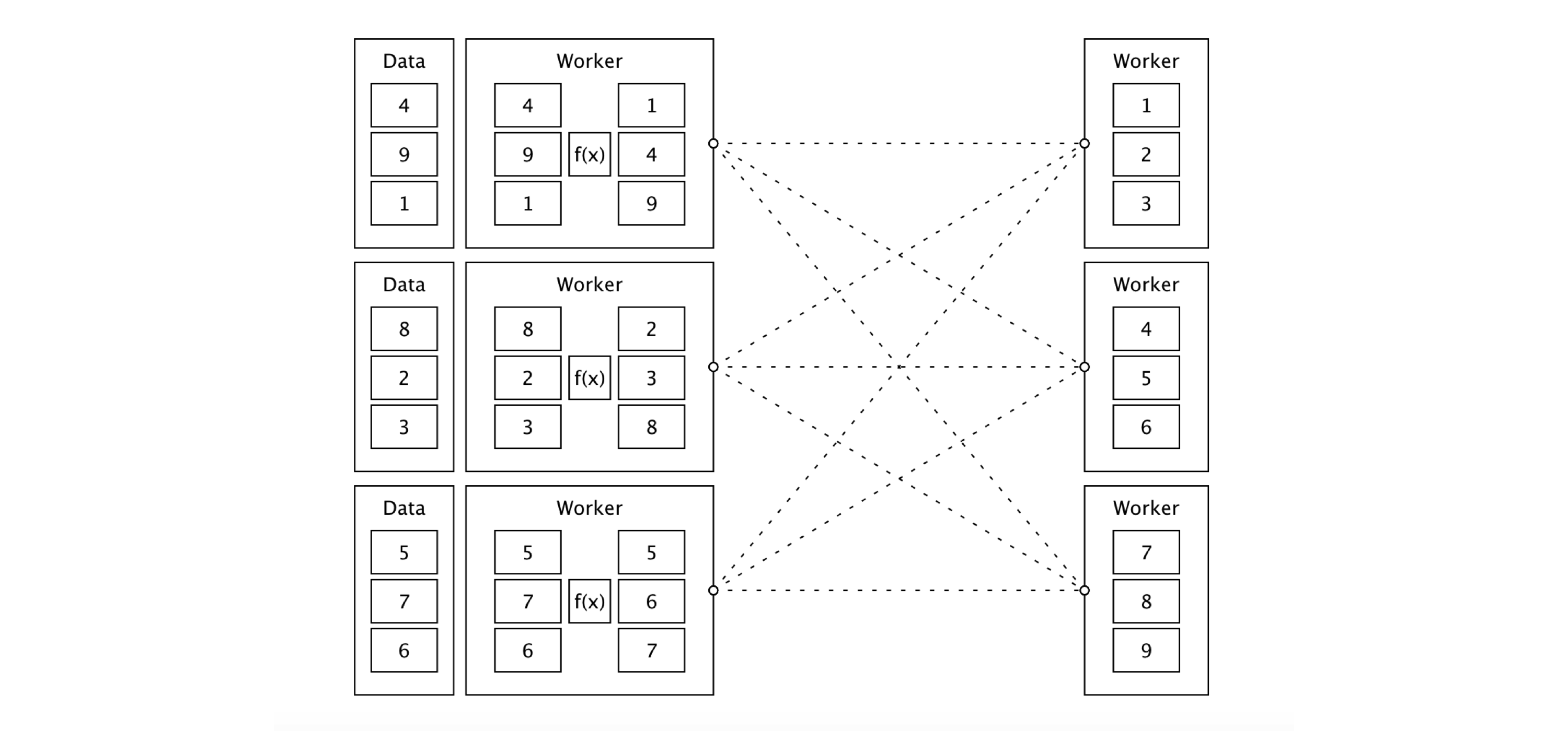 FIGURE 9.1: Sorting distributed data with Apache Spark
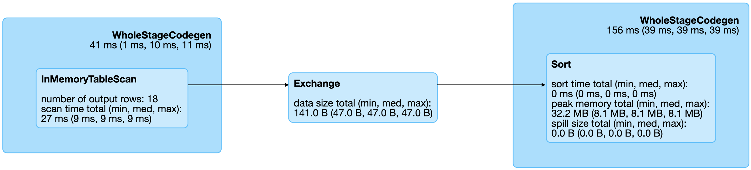 FIGURE 9.2: Spark graph for a sorting query
From the query details, you then can open the last Spark job to arrive to the job details page, which you can expand by using “DAG Visualization” to create a graph similar to Figure 9.3.
This graph shows a few additional details and the stages in this job.
Notice that there are no arrows pointing back to previous steps, since Spark makes use of acyclic graphs.
FIGURE 9.2: Spark graph for a sorting query
From the query details, you then can open the last Spark job to arrive to the job details page, which you can expand by using “DAG Visualization” to create a graph similar to Figure 9.3.
This graph shows a few additional details and the stages in this job.
Notice that there are no arrows pointing back to previous steps, since Spark makes use of acyclic graphs.
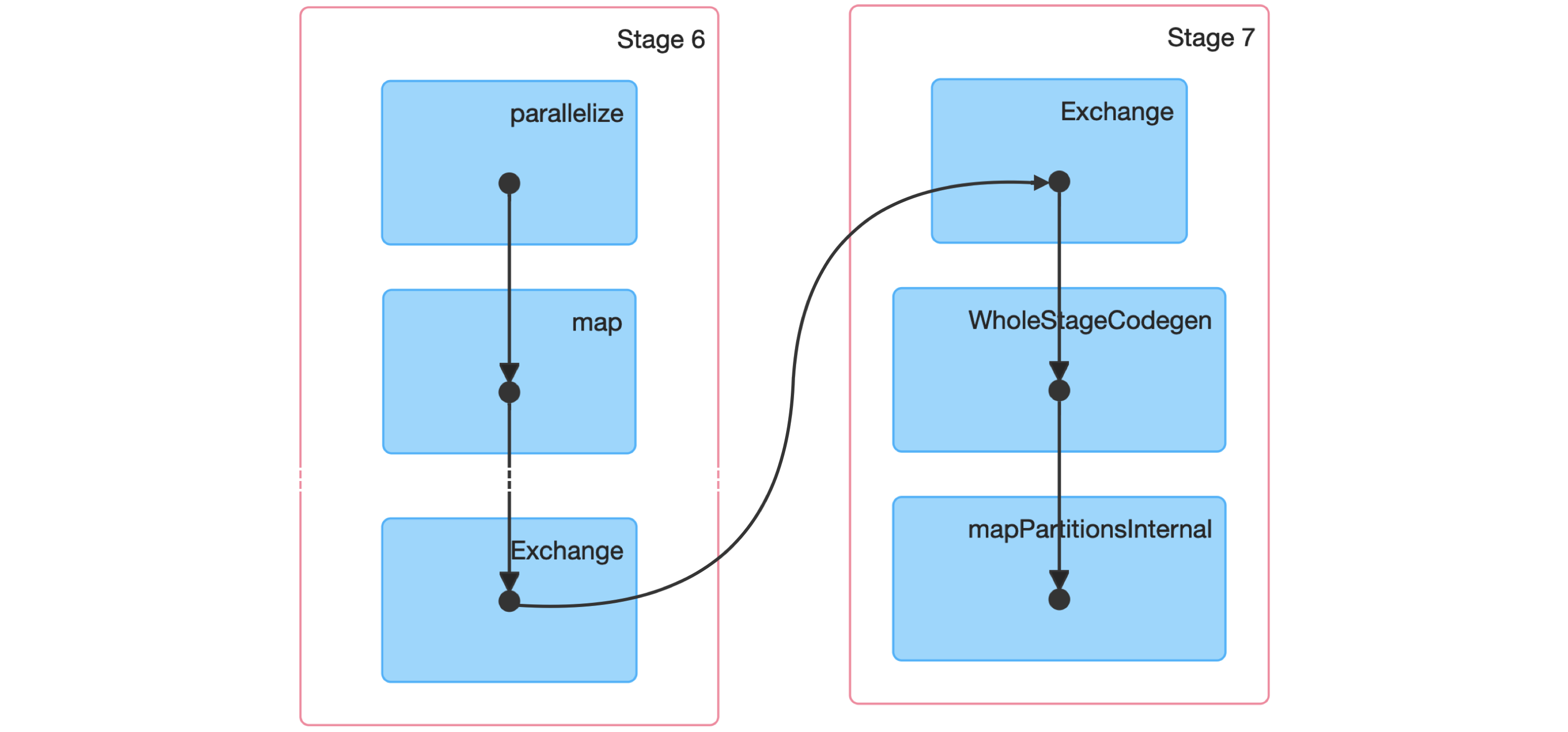 FIGURE 9.3: Spark graph for a sorting job
Next, we dive into a Spark stage and explore its event timeline.
FIGURE 9.3: Spark graph for a sorting job
Next, we dive into a Spark stage and explore its event timeline.
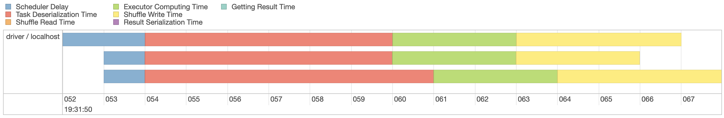 FIGURE 9.4: Spark event timeline
Since our machine is equipped with four CPUs, we can(((“parallel execution”))) parallelize this computation even further by explicitly repartitioning data using
FIGURE 9.4: Spark event timeline
Since our machine is equipped with four CPUs, we can(((“parallel execution”))) parallelize this computation even further by explicitly repartitioning data using 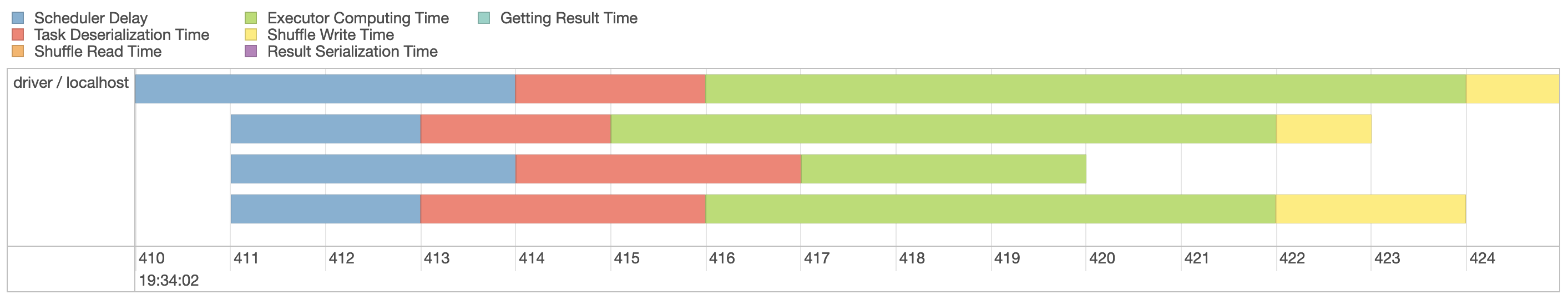 FIGURE 9.5: Spark event timeline with additional partitions
Figure 9.5 now shows four execution lanes with most time spent under Executor Computing Time, which shows us that this particular operation is making better use of our compute resources.
When you are working with clusters, requesting more compute nodes from your cluster should shorten computation time.
In contrast, for timelines that show significant time spent shuffling, requesting more compute nodes might not shorten time and might actually make everything slower.
There is no concrete set of rules to follow to optimize a stage; however, as you gain experience understanding this timeline over multiple operations, you will develop insights as to how to properly optimize Spark operations.
FIGURE 9.5: Spark event timeline with additional partitions
Figure 9.5 now shows four execution lanes with most time spent under Executor Computing Time, which shows us that this particular operation is making better use of our compute resources.
When you are working with clusters, requesting more compute nodes from your cluster should shorten computation time.
In contrast, for timelines that show significant time spent shuffling, requesting more compute nodes might not shorten time and might actually make everything slower.
There is no concrete set of rules to follow to optimize a stage; however, as you gain experience understanding this timeline over multiple operations, you will develop insights as to how to properly optimize Spark operations.
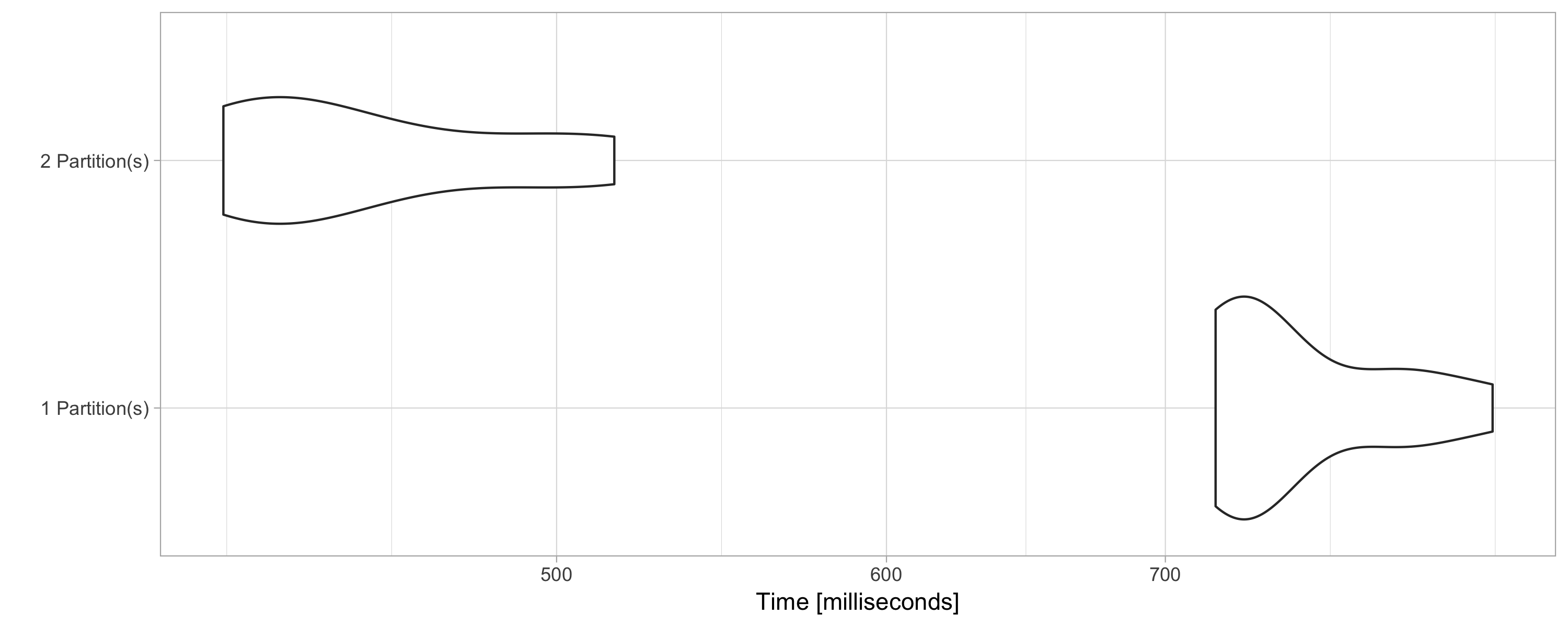 FIGURE 9.6: Computation speed with additional explicit partitions
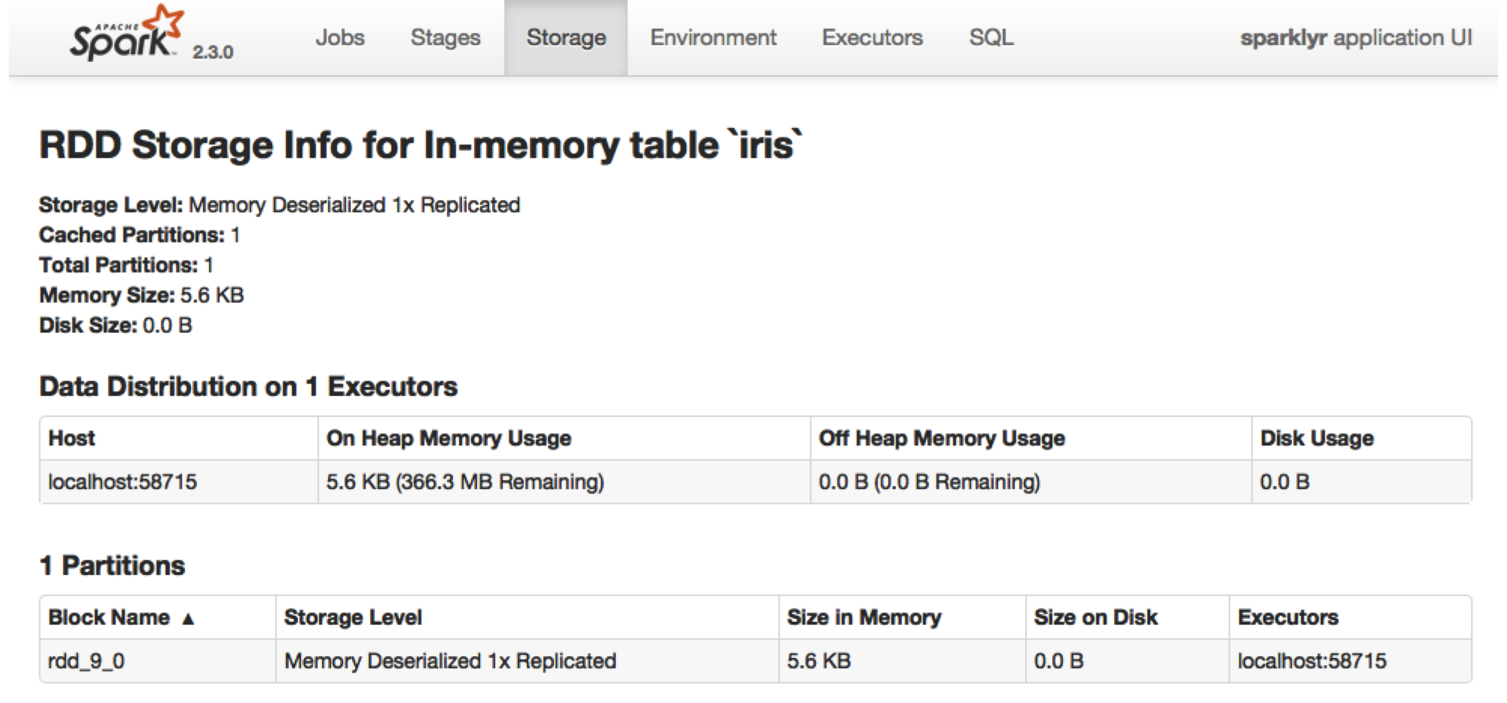 FIGURE 9.7: Cached RDD in the Spark web interface
Data loaded in memory will be released when the R session terminates, either explicitly or implicitly, with a restart or disconnection; however, to free up resources, you can use
FIGURE 9.7: Cached RDD in the Spark web interface
Data loaded in memory will be released when the R session terminates, either explicitly or implicitly, with a restart or disconnection; however, to free up resources, you can use 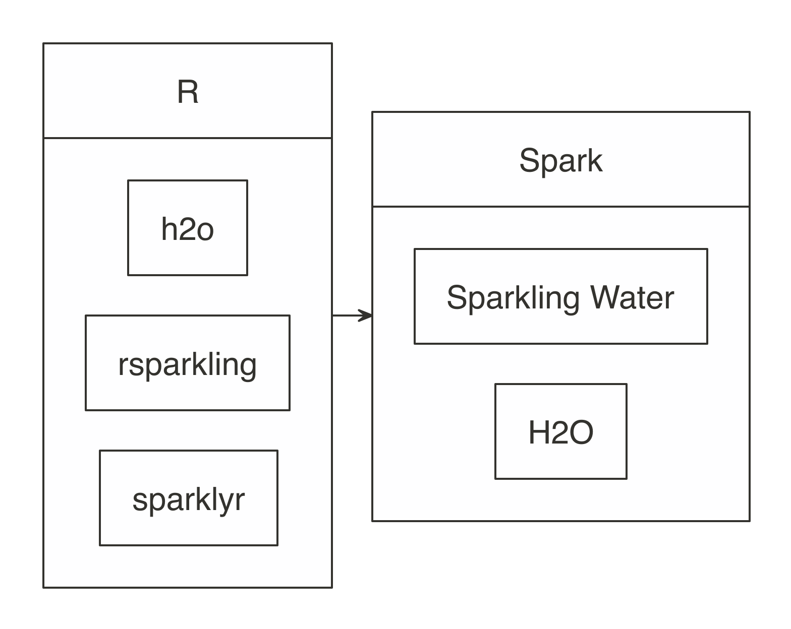 FIGURE 10.1: H2O components with Spark and R
First, install
FIGURE 10.1: H2O components with Spark and R
First, install 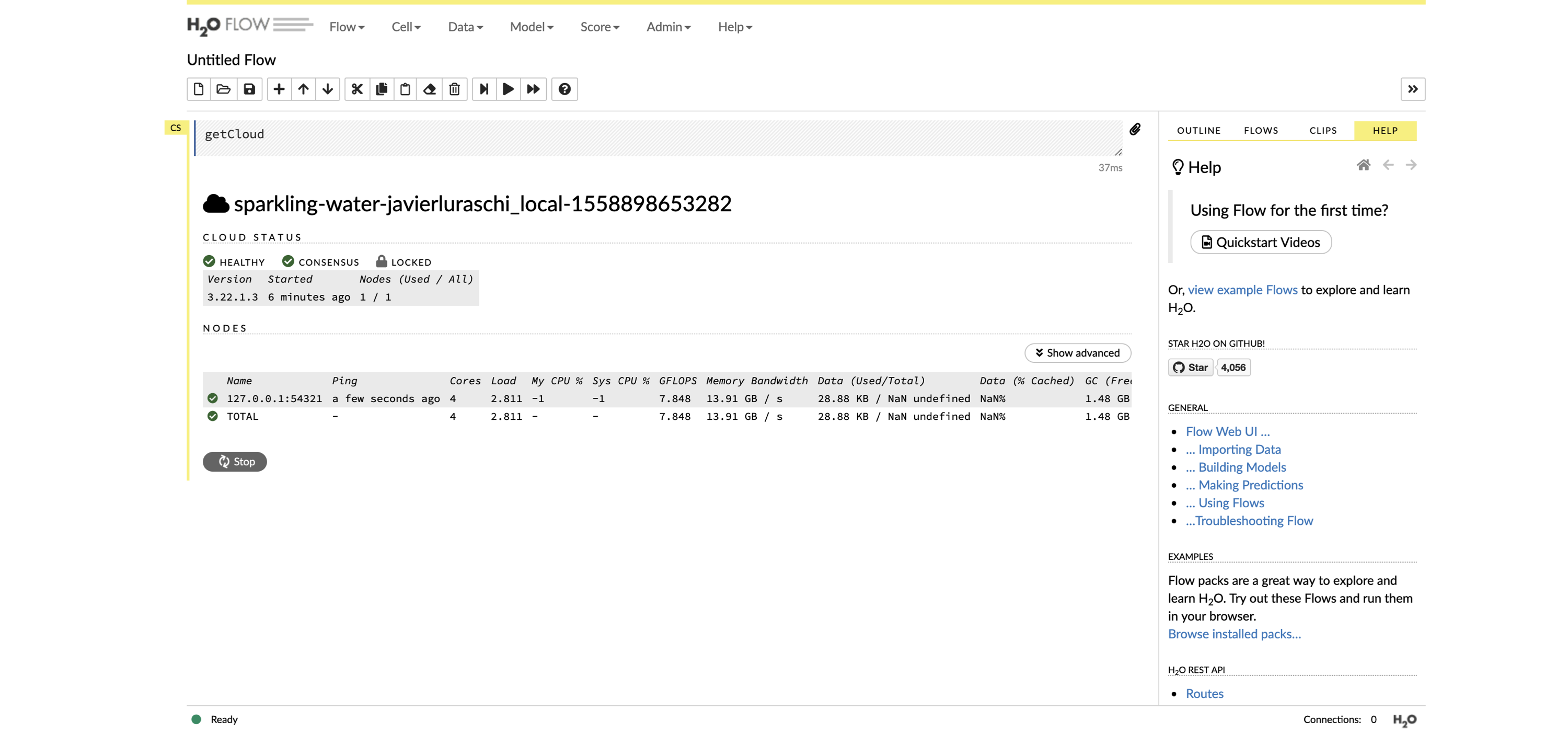 FIGURE 10.2: The H2O Flow interface using Spark with R
Then, you can use many of the modeling functions available in the
FIGURE 10.2: The H2O Flow interface using Spark with R
Then, you can use many of the modeling functions available in the  FIGURE 10.3: The Seven Bridges of Königsberg from the Euler archive
Today, a graph is defined as an ordered pair
FIGURE 10.3: The Seven Bridges of Königsberg from the Euler archive
Today, a graph is defined as an ordered pair 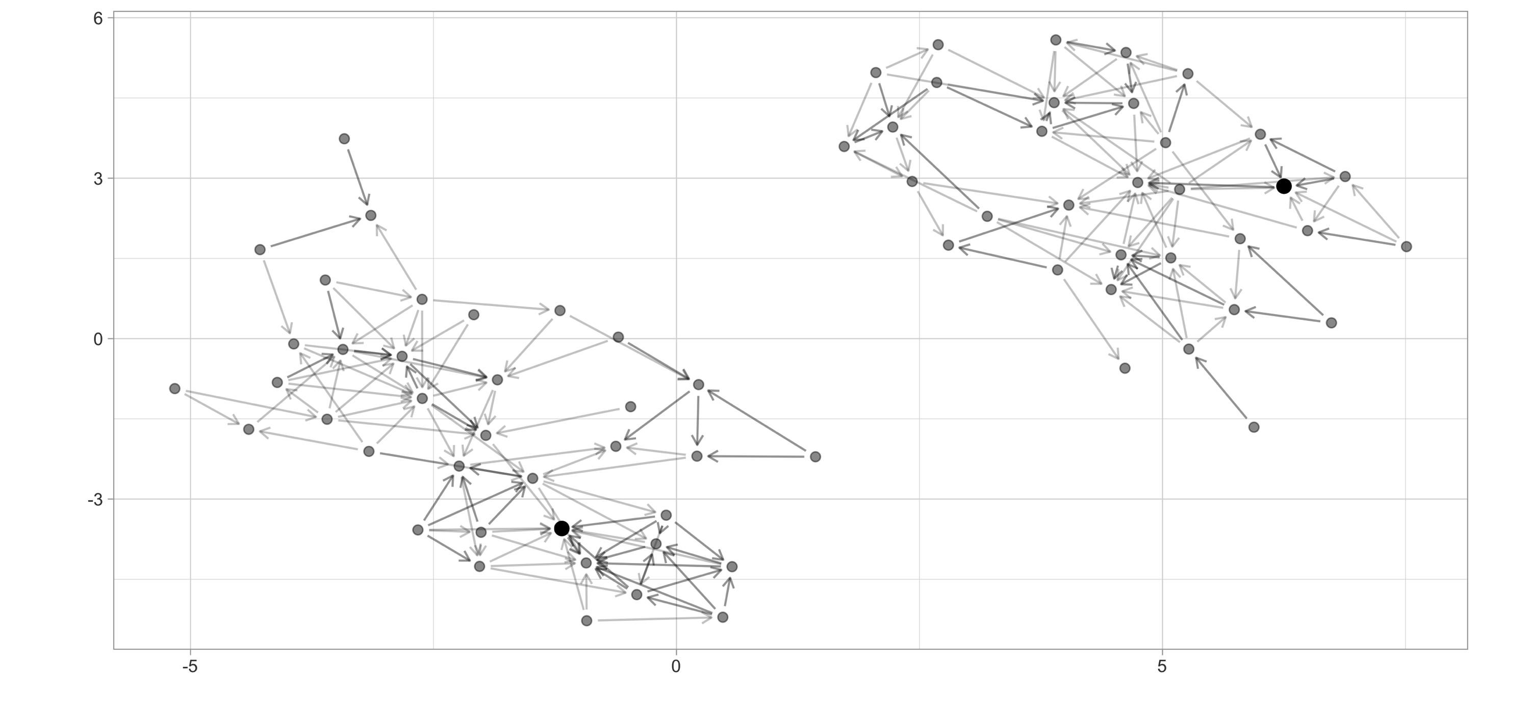 FIGURE 10.4: High school ggraph dataset with highest PageRank highlighted
There are many more graph algorithms provided in
FIGURE 10.4: High school ggraph dataset with highest PageRank highlighted
There are many more graph algorithms provided in 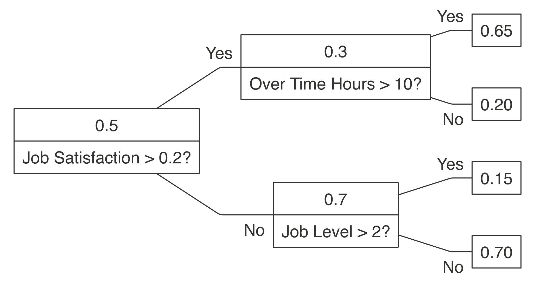 FIGURE 10.5: A decision tree to predict job attrition based on known factors
While a decision tree representation is quite easy to understand and to interpret, finding out the decisions in the tree requires mathematical techniques like gradient descent to find a local minimum.
Gradient descent takes steps proportional to the negative of the gradient of the function at the current point.
The gradient is represented by
FIGURE 10.5: A decision tree to predict job attrition based on known factors
While a decision tree representation is quite easy to understand and to interpret, finding out the decisions in the tree requires mathematical techniques like gradient descent to find a local minimum.
Gradient descent takes steps proportional to the negative of the gradient of the function at the current point.
The gradient is represented by 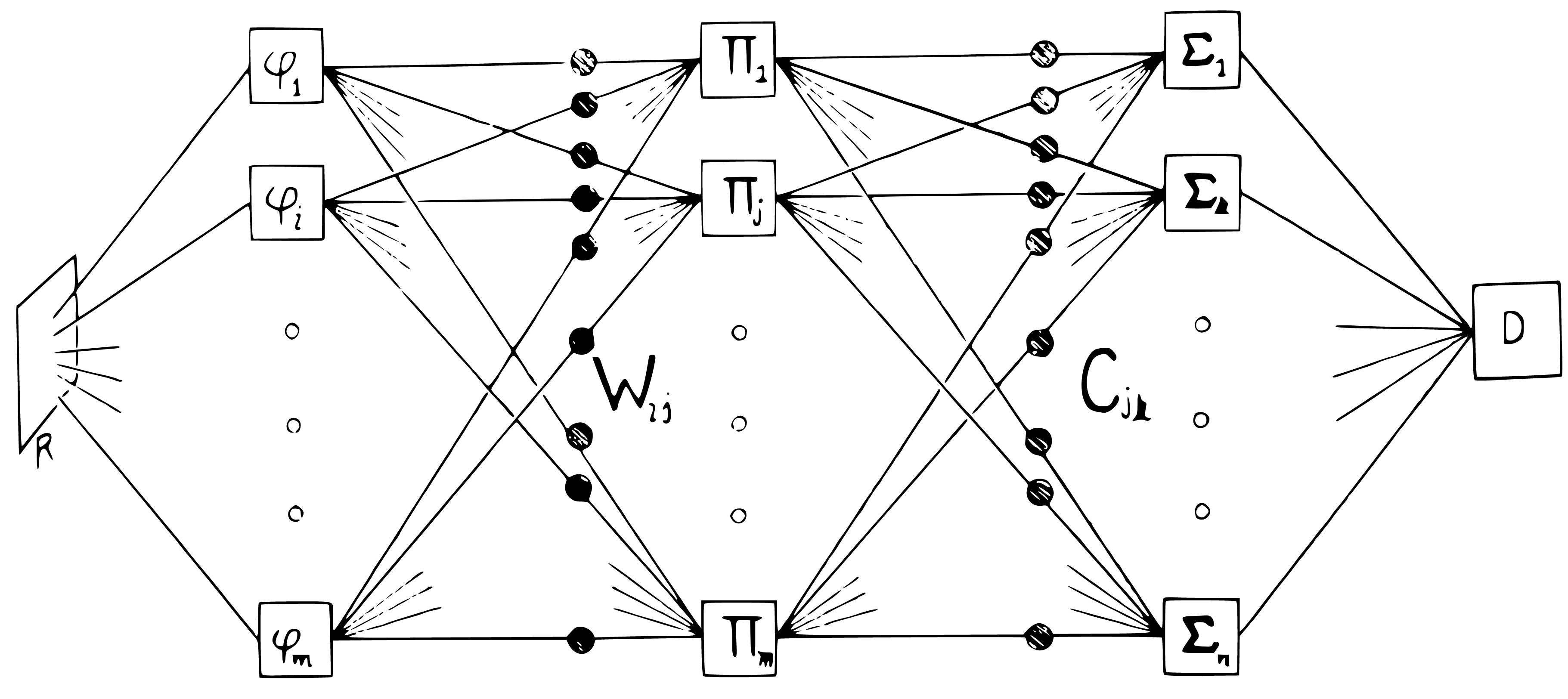 FIGURE 10.6: Layered perceptrons, as illustrated in the book Perceptrons
Before we start, let’s first install all the packages that we are about to use:
FIGURE 10.6: Layered perceptrons, as illustrated in the book Perceptrons
Before we start, let’s first install all the packages that we are about to use:
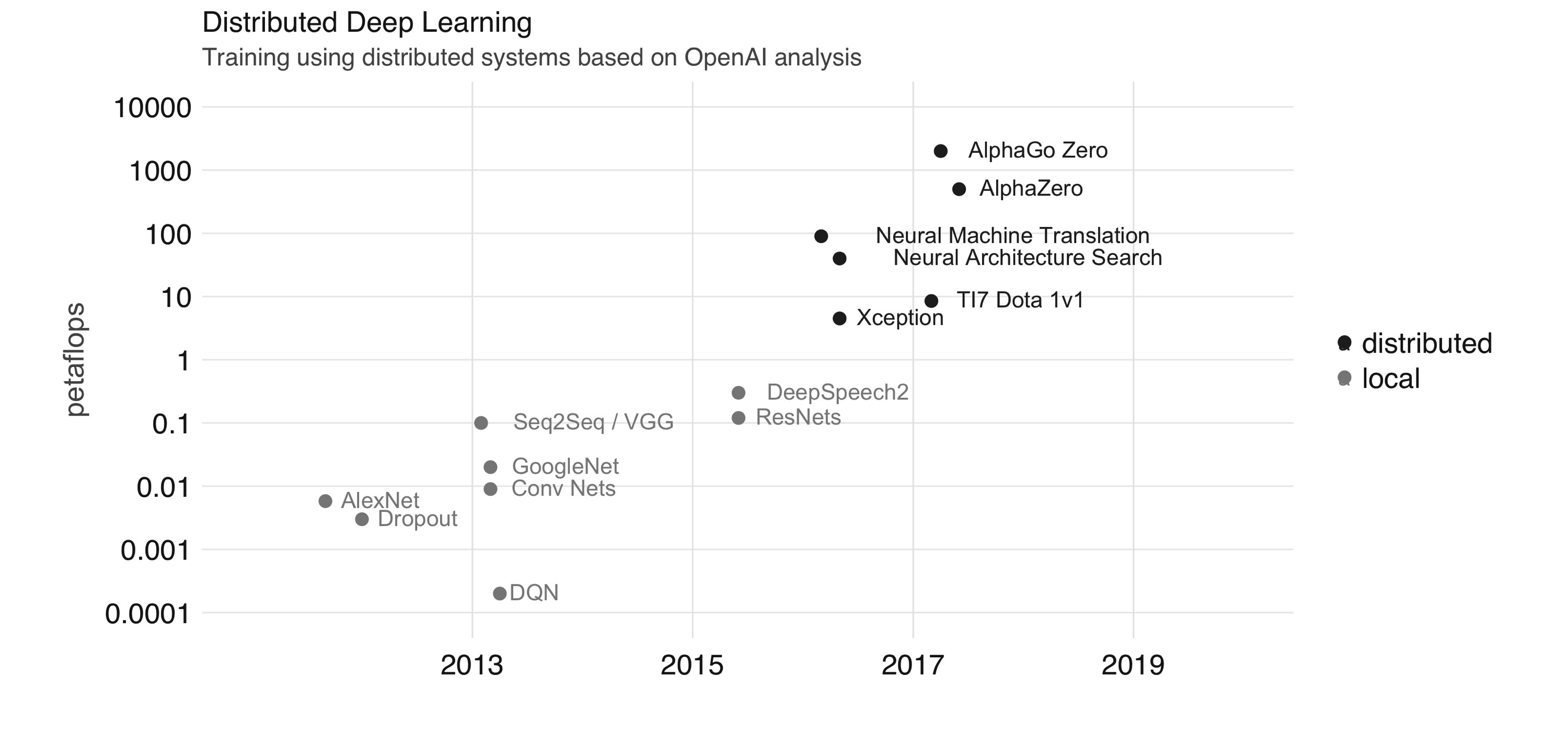 FIGURE 10.7: Training using distributed systems based on OpenAI analysis
Training large-scale deep learning models is possible in Spark and TensorFlow through frameworks like Horovod.
Today, it’s possible to use Horovod with Spark from R using the
FIGURE 10.7: Training using distributed systems based on OpenAI analysis
Training large-scale deep learning models is possible in Spark and TensorFlow through frameworks like Horovod.
Today, it’s possible to use Horovod with Spark from R using the 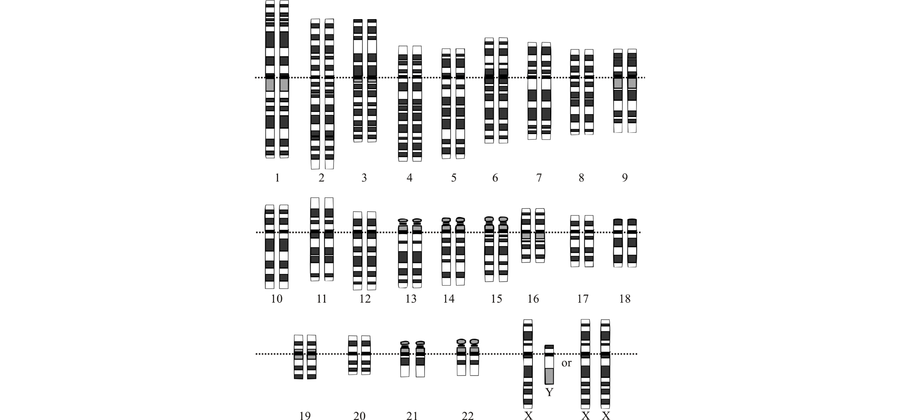 FIGURE 10.8: The idealized human diploid karyotype showing the organization of the genome into chromosomes
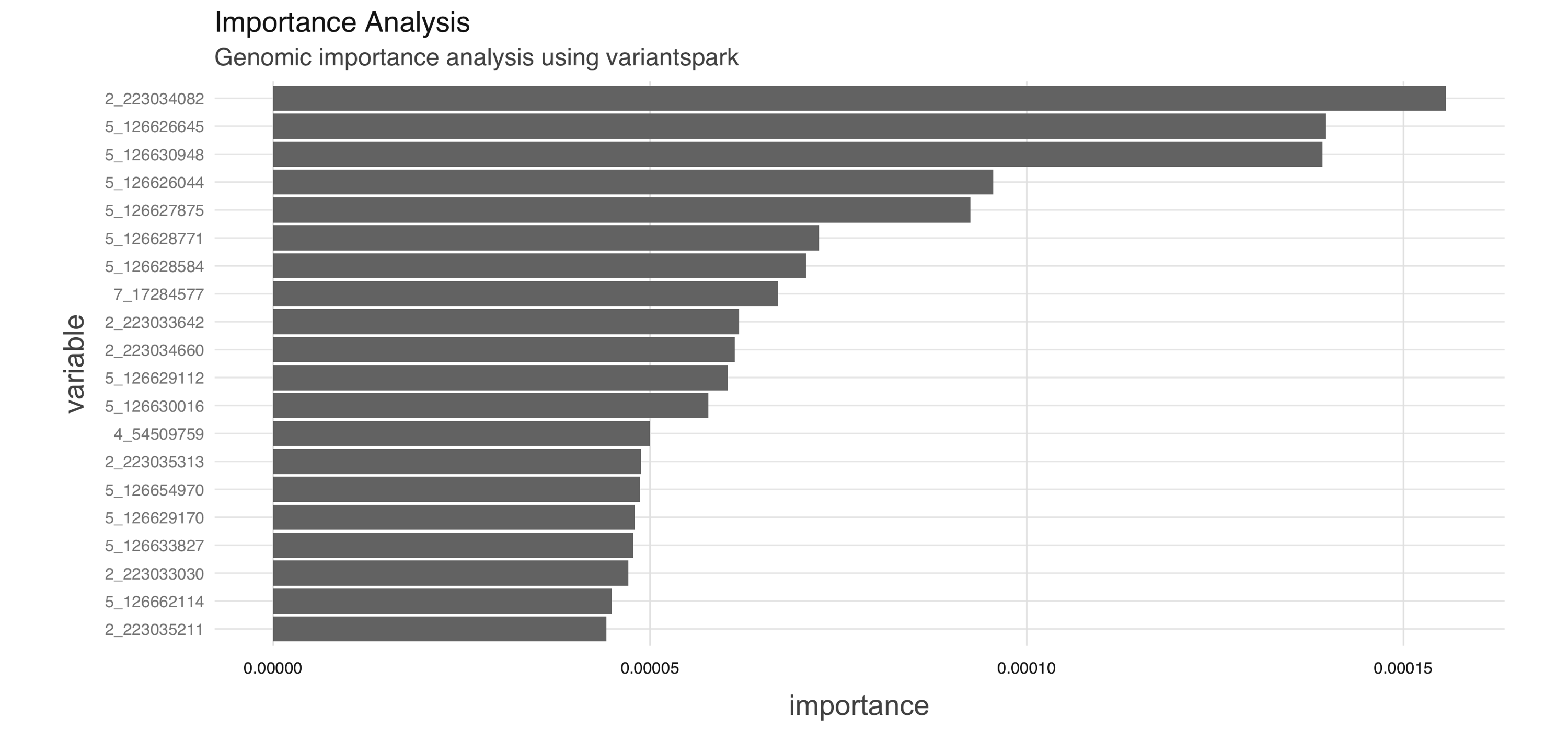 FIGURE 10.9: Genomic importance analysis using variantspark
This concludes a brief introduction to genomic analysis in Spark using the
FIGURE 10.9: Genomic importance analysis using variantspark
This concludes a brief introduction to genomic analysis in Spark using the 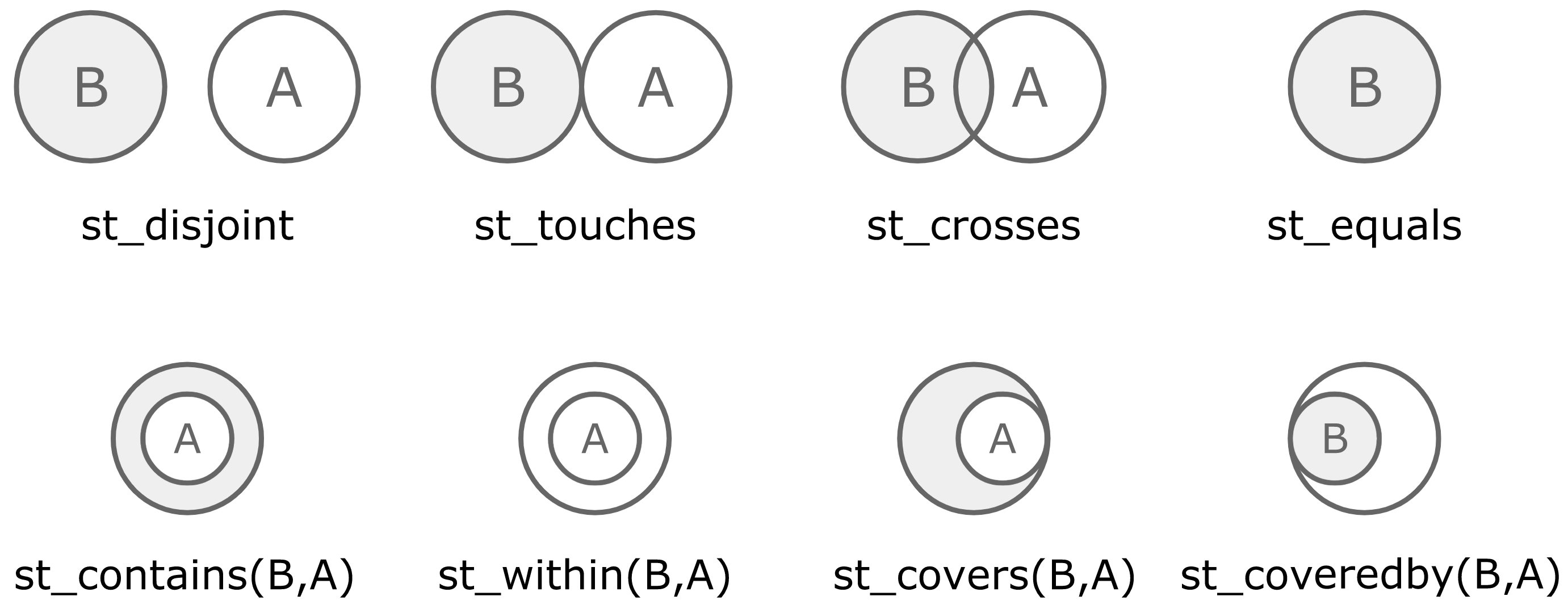 FIGURE 10.10: Spatial operations available in geospark
For instance, we can use these operations to find the polygons that contain a given set of points using
FIGURE 10.10: Spatial operations available in geospark
For instance, we can use these operations to find the polygons that contain a given set of points using 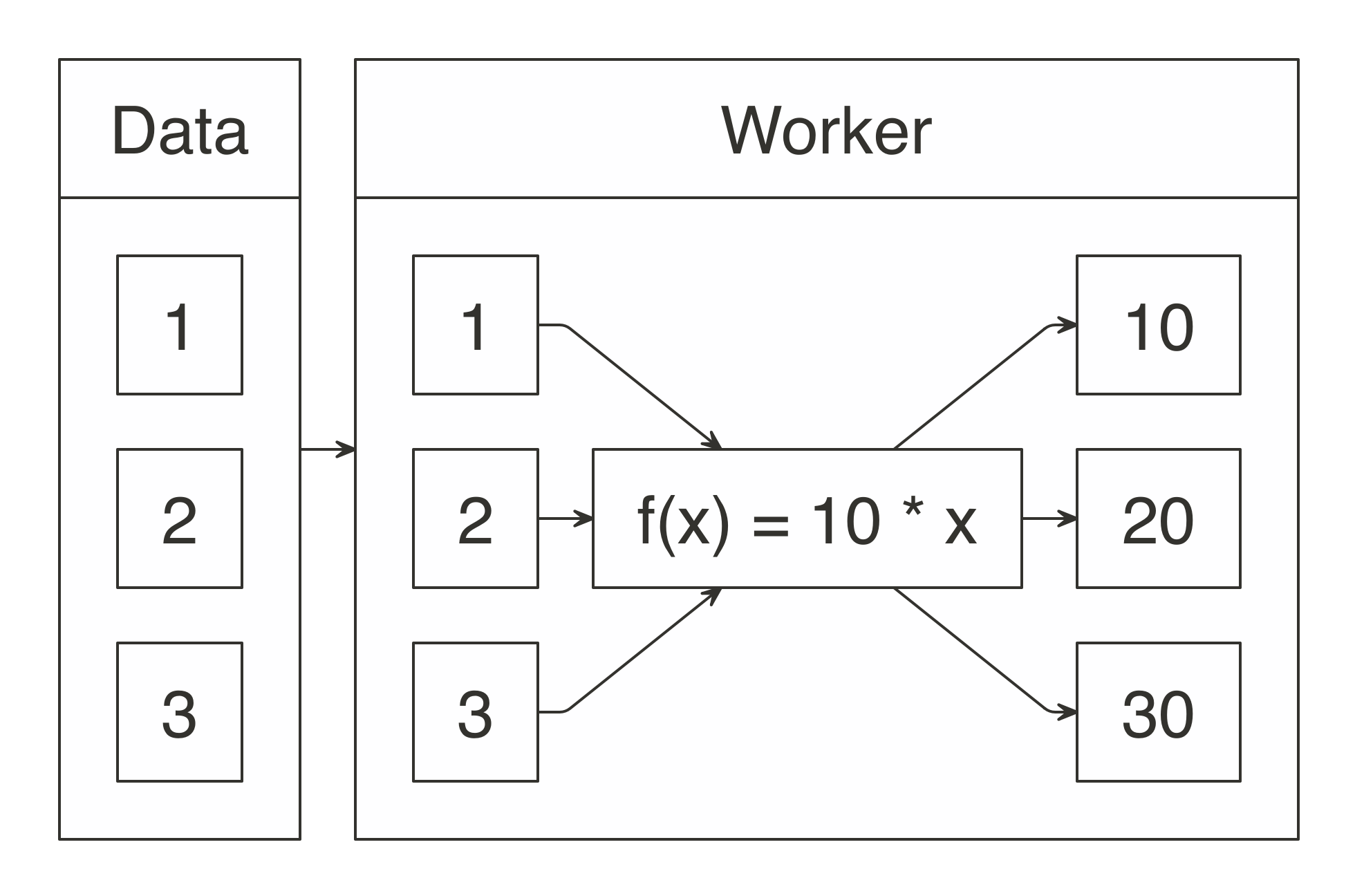 FIGURE 11.1: Map operation when multiplying by 10
This chapter presents how to define a custom
FIGURE 11.1: Map operation when multiplying by 10
This chapter presents how to define a custom 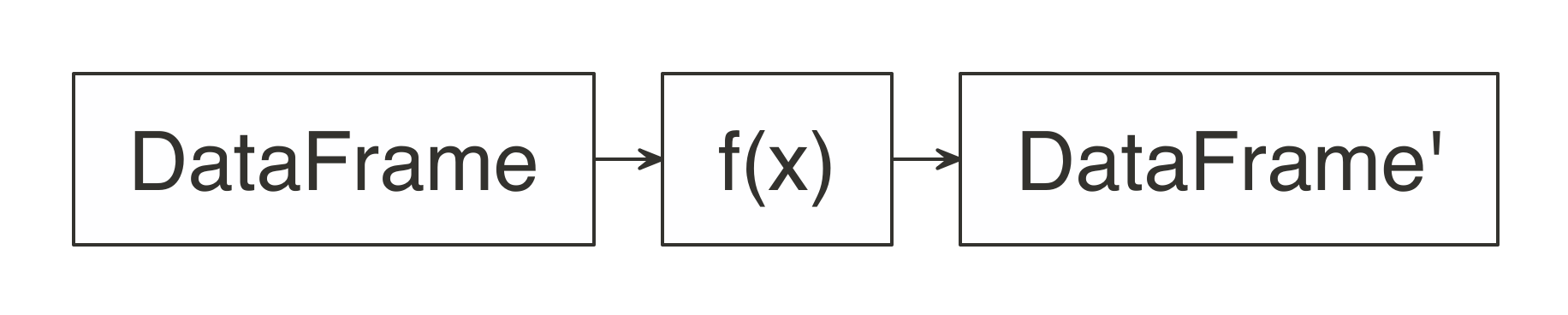 FIGURE 11.2: Expected function signature in spark_apply() mappings
We can refer back to the original MapReduce example from Chapter 1, where the map operation was defined to split sentences into words and the total unique words were counted as the reduce operation.
In R, we could make use of the
FIGURE 11.2: Expected function signature in spark_apply() mappings
We can refer back to the original MapReduce example from Chapter 1, where the map operation was defined to split sentences into words and the total unique words were counted as the reduce operation.
In R, we could make use of the 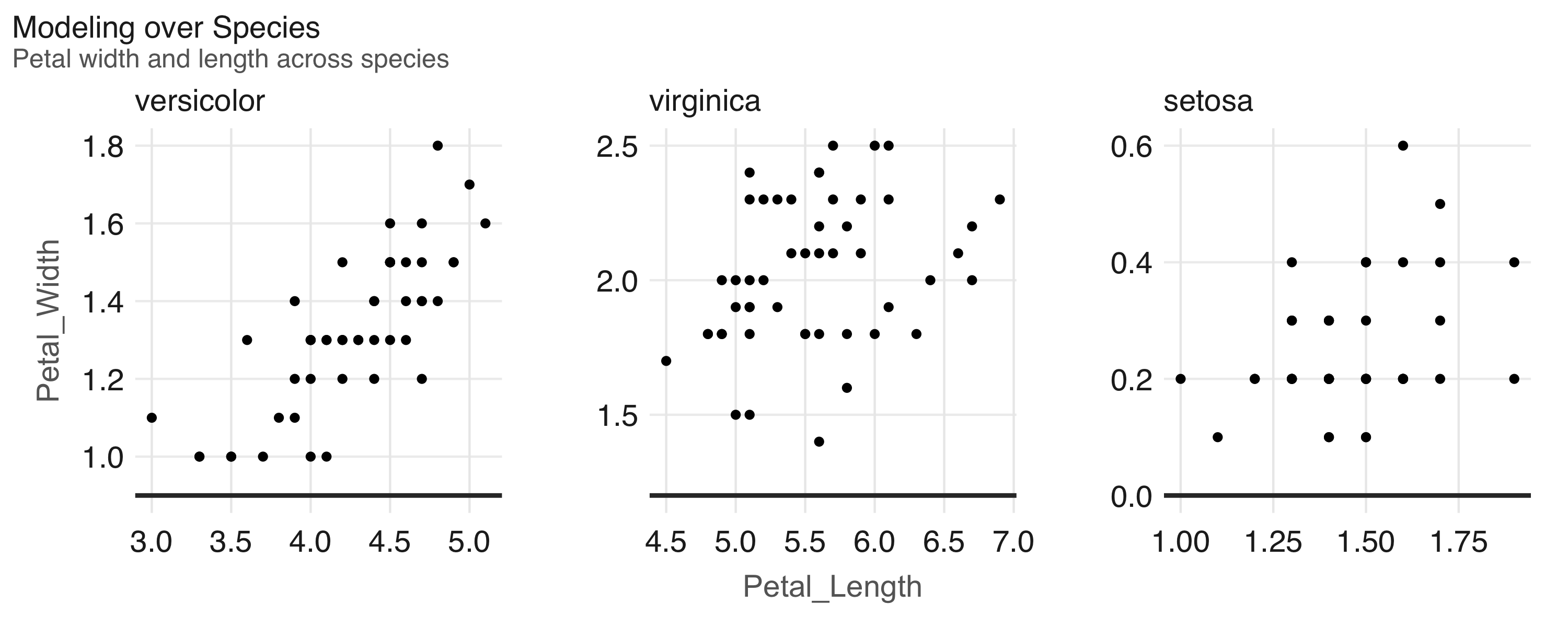 FIGURE 11.3: Modeling over species in the iris dataset
This concludes our brief overview on how to perform modeling over several different partitionable datasets.
A similar technique can be applied to perform modeling over the same dataset using different modeling parameters, as we cover next.
FIGURE 11.3: Modeling over species in the iris dataset
This concludes our brief overview on how to perform modeling over several different partitionable datasets.
A similar technique can be applied to perform modeling over the same dataset using different modeling parameters, as we cover next.
 FIGURE 11.4: Ray tracing in Spark using R and rayrender
In higher resolutions, say 1920 x 1080, the previous example takes several minutes to render the single frame from Figure 11.4; rendering a few seconds at 30 frames per second would take several hours in a single machine.
However, we can reduce this time using multiple machines by parallelizing computation across them.
For instance, using 10 machines with the same number of CPUs would cut rendering time tenfold:
FIGURE 11.4: Ray tracing in Spark using R and rayrender
In higher resolutions, say 1920 x 1080, the previous example takes several minutes to render the single frame from Figure 11.4; rendering a few seconds at 30 frames per second would take several hours in a single machine.
However, we can reduce this time using multiple machines by parallelizing computation across them.
For instance, using 10 machines with the same number of CPUs would cut rendering time tenfold:
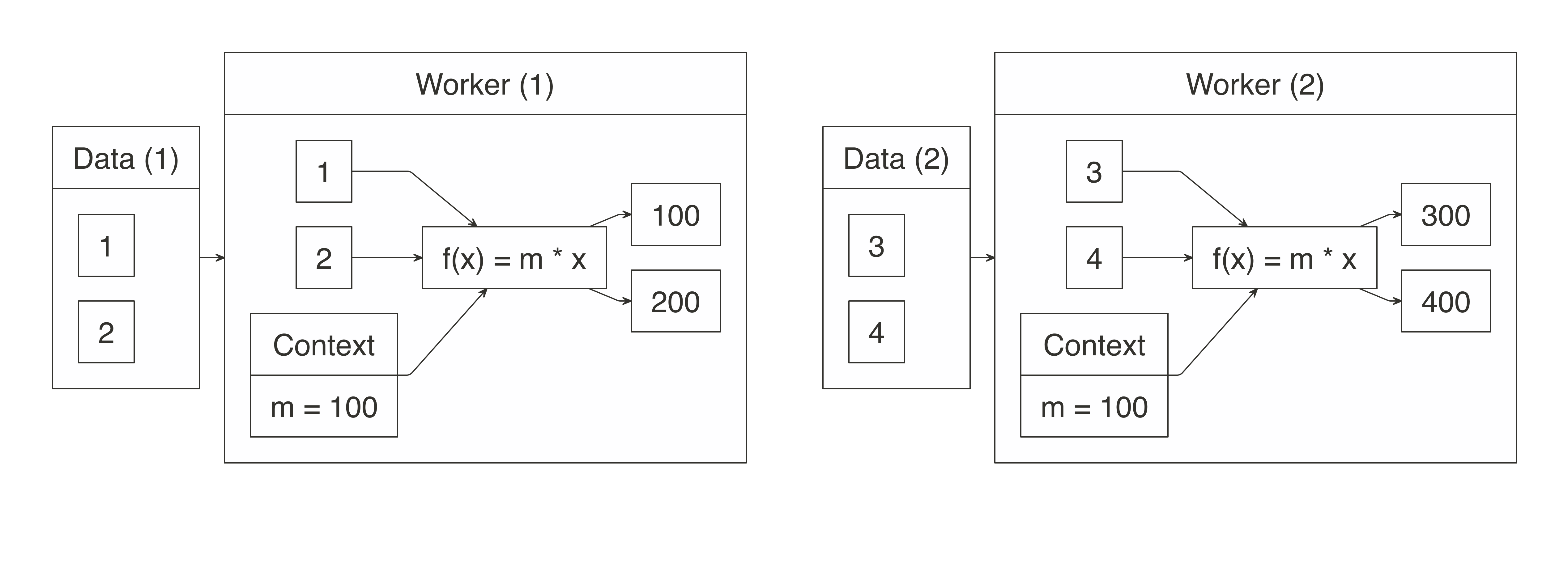 FIGURE 11.5: Map operation when multiplying with context
The grid search example used this parameter to pass a DataFrame to each worker node; however, since the context parameter is serialized as an R object, it can contain anything.
For instance, if you need to pass multiple values—or even multiple datasets—you can pass a list with values.
The following example defines a
FIGURE 11.5: Map operation when multiplying with context
The grid search example used this parameter to pass a DataFrame to each worker node; however, since the context parameter is serialized as an R object, it can contain anything.
For instance, if you need to pass multiple values—or even multiple datasets—you can pass a list with values.
The following example defines a 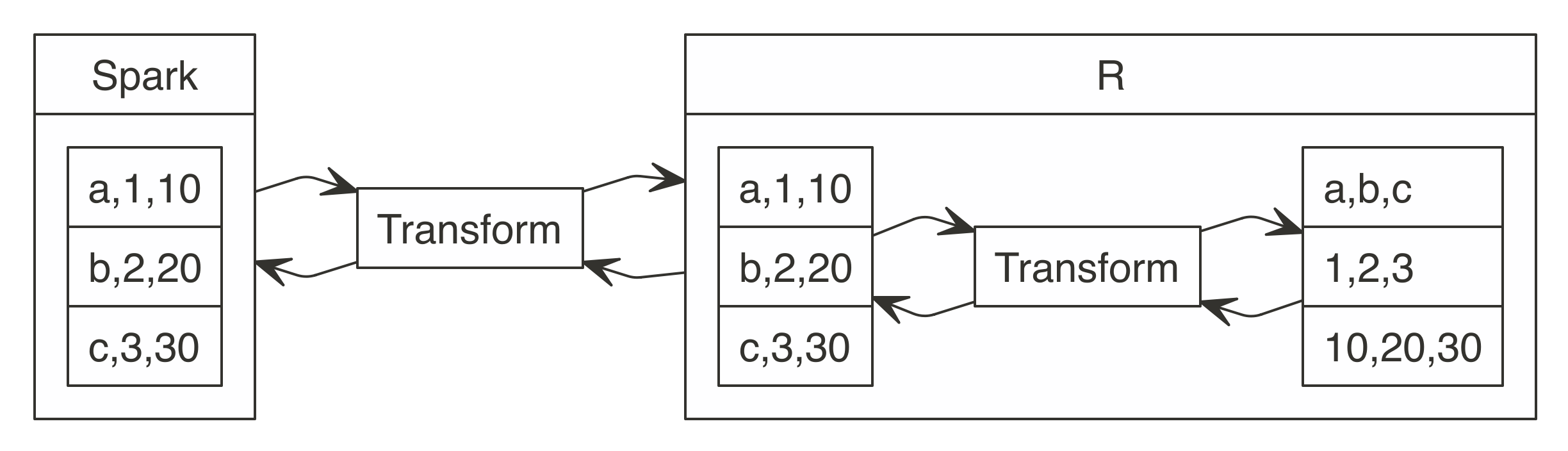 FIGURE 11.6: Data transformation between Spark and R
This transformation from rows to columns needs to happen for each partition.
In addition, data also must be transformed from Scala’s internal representation to R’s internal representation.
Apache Arrow reduces these transformations that waste a lot of CPU cycles.
Apache Arrow is a cross-language development platform for in-memory data.
In Spark, it speeds up transferring data between Scala and R by defining a common data format compatible with many programming languages.
Instead of having to transform between Scala’s internal representation and R’s, you can use the same structure for both languages.
In addition, transforming data from row-based storage to columnar storage is performed in parallel in Spark, which can be further optimized by using the columnar storage formats presented in Chapter 8.
The improved transformations are shown in Figure 11.6.
FIGURE 11.6: Data transformation between Spark and R
This transformation from rows to columns needs to happen for each partition.
In addition, data also must be transformed from Scala’s internal representation to R’s internal representation.
Apache Arrow reduces these transformations that waste a lot of CPU cycles.
Apache Arrow is a cross-language development platform for in-memory data.
In Spark, it speeds up transferring data between Scala and R by defining a common data format compatible with many programming languages.
Instead of having to transform between Scala’s internal representation and R’s, you can use the same structure for both languages.
In addition, transforming data from row-based storage to columnar storage is performed in parallel in Spark, which can be further optimized by using the columnar storage formats presented in Chapter 8.
The improved transformations are shown in Figure 11.6.
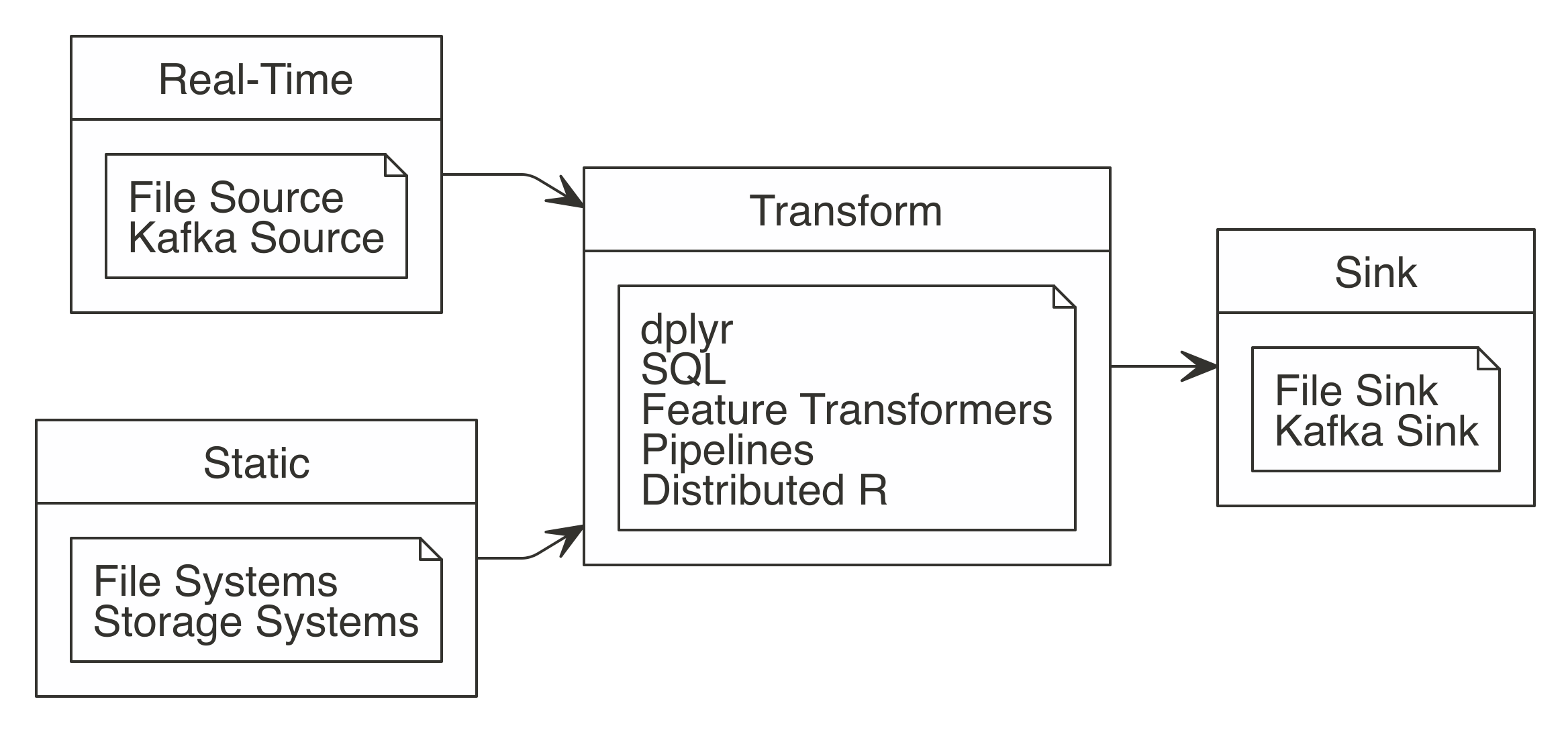 FIGURE 12.1: Working with Spark Streaming
Let’s take a look at each of these a little more closely:
FIGURE 12.1: Working with Spark Streaming
Let’s take a look at each of these a little more closely:
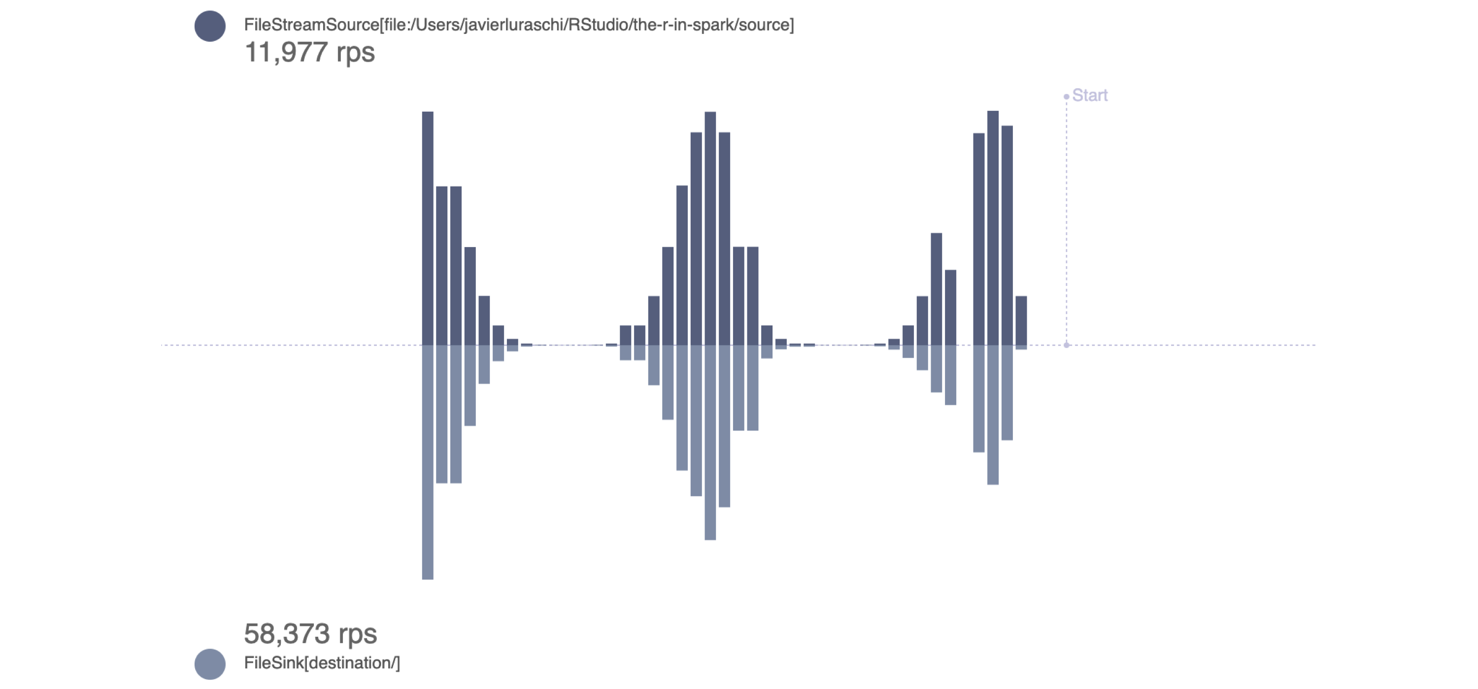 FIGURE 12.2: Monitoring a stream generating rows following a binomial distribution
Notice that the rps rate in the destination stream is higher than that in the source stream.
This is expected and desirable since Spark measures incoming rates from the source stream, but also actual row-processing times in the destination stream.
For example, if 10 rows per second are written to the source/ path, the incoming rate is 10 rps.
However, if it takes Spark only 0.01 seconds to write all those 10 rows, the output rate is 100 rps.
Use
FIGURE 12.2: Monitoring a stream generating rows following a binomial distribution
Notice that the rps rate in the destination stream is higher than that in the source stream.
This is expected and desirable since Spark measures incoming rates from the source stream, but also actual row-processing times in the destination stream.
For example, if 10 rows per second are written to the source/ path, the incoming rate is 10 rps.
However, if it takes Spark only 0.01 seconds to write all those 10 rows, the output rate is 100 rps.
Use 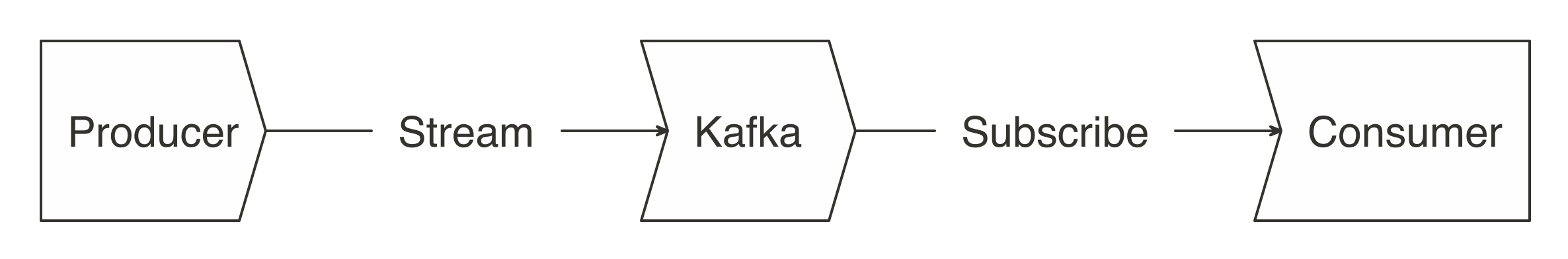 FIGURE 12.3: A basic Kafka workflow
If you are new to Kafka, we don’t recommend you run the code from this section.
However, if you’re really motivated to follow along, you will first need to install Kafka as explained in Appendix or deploy it in your cluster.
Using Kafka also requires you to have the Kafka package when connecting to Spark.
Make sure this is specified in your connection
FIGURE 12.3: A basic Kafka workflow
If you are new to Kafka, we don’t recommend you run the code from this section.
However, if you’re really motivated to follow along, you will first need to install Kafka as explained in Appendix or deploy it in your cluster.
Using Kafka also requires you to have the Kafka package when connecting to Spark.
Make sure this is specified in your connection 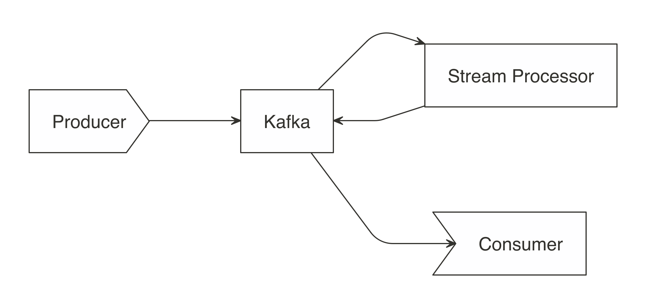 FIGURE 12.4: A Kafka workflow using stream processors
Three modes are available when processing Kafka streams in Spark: complete, update, and append.
The
FIGURE 12.4: A Kafka workflow using stream processors
Three modes are available when processing Kafka streams in Spark: complete, update, and append.
The 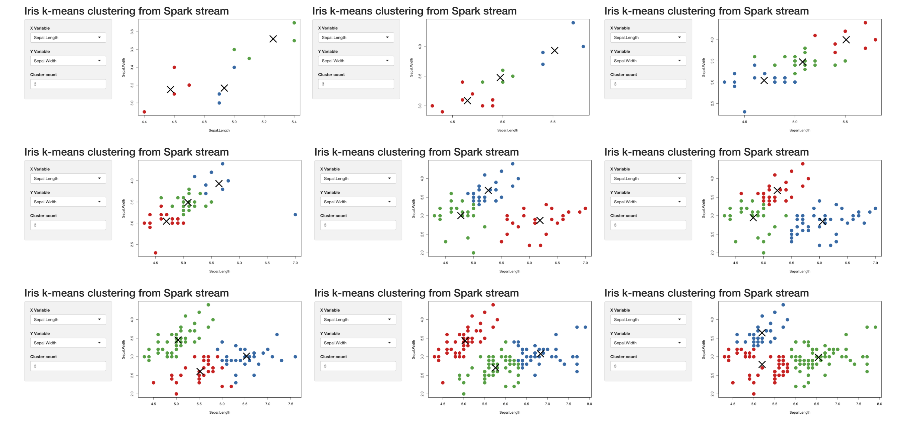 FIGURE 12.5: Progression of Spark reactive loading data into the Shiny app
In this section you learned how easy it is to create a Shiny app that can be used for several different purposes, such as monitoring and dashboarding.
In a more complex implementation, the source would more likely be a Kafka stream.
Before we transition, disconnect from Spark and clear the folders that we used:
FIGURE 12.5: Progression of Spark reactive loading data into the Shiny app
In this section you learned how easy it is to create a Shiny app that can be used for several different purposes, such as monitoring and dashboarding.
In a more complex implementation, the source would more likely be a Kafka stream.
Before we transition, disconnect from Spark and clear the folders that we used:
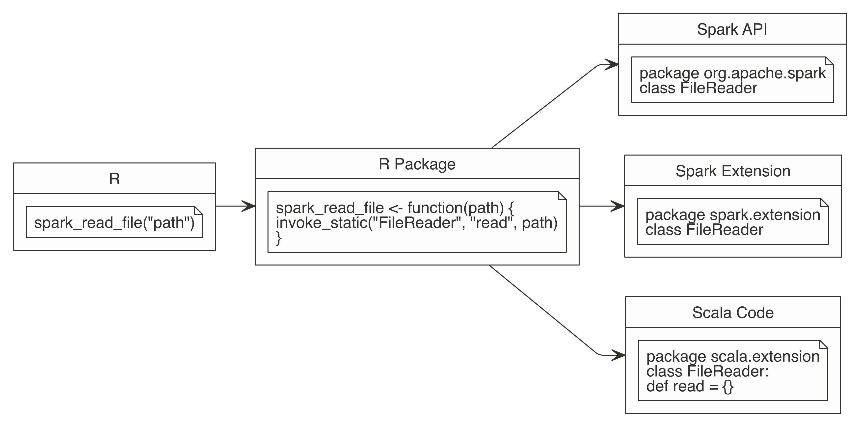 FIGURE 13.1: Extending Spark using the Spark API or Spark extensions, or writing Scala code
We will focus first on extending Spark using the Spark API, since the techniques required to call the Spark API are also applicable while calling Spark extensions or custom Scala code.
FIGURE 13.1: Extending Spark using the Spark API or Spark extensions, or writing Scala code
We will focus first on extending Spark using the Spark API, since the techniques required to call the Spark API are also applicable while calling Spark extensions or custom Scala code.
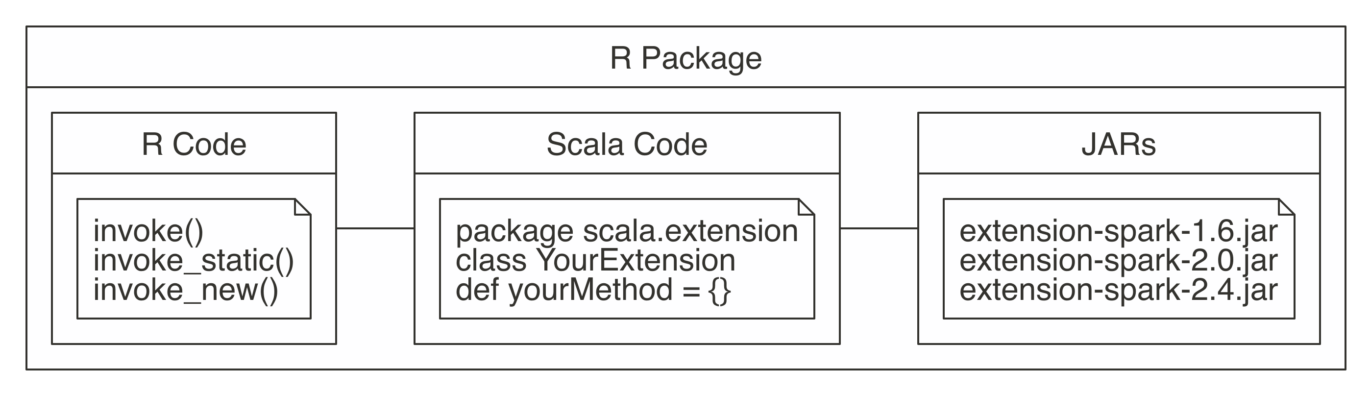 FIGURE 13.2: R package structure when using Scala code
As usual, the R code should be placed under a top-level R folder, Scala code under a java folder, and the compiled JARs under an inst/java folder.
Though you are certainly welcome to manually compile the Scala code, you can use helper functions to download the required compiler and compile Scala code.
To compile Scala code, you’ll need to install the Java Development Kit 8 (JDK8, for short).
Download the JDK from Oracle’s Java download page; this will require you to restart your R session.
You’ll also need a Scala compiler for Scala 2.11 and 2.12.
The Scala compilers can be automatically downloaded and installed using
FIGURE 13.2: R package structure when using Scala code
As usual, the R code should be placed under a top-level R folder, Scala code under a java folder, and the compiled JARs under an inst/java folder.
Though you are certainly welcome to manually compile the Scala code, you can use helper functions to download the required compiler and compile Scala code.
To compile Scala code, you’ll need to install the Java Development Kit 8 (JDK8, for short).
Download the JDK from Oracle’s Java download page; this will require you to restart your R session.
You’ll also need a Scala compiler for Scala 2.11 and 2.12.
The Scala compilers can be automatically downloaded and installed using  FIGURE 13.3: Creating a Scala extension package from RStudio
Once you are ready to compile your package JARs, you can simply run the following:
FIGURE 13.3: Creating a Scala extension package from RStudio
Once you are ready to compile your package JARs, you can simply run the following:
 FIGURE 14.1: The R Project for Statistical Computing
 FIGURE 14.2: Java Download Page
Starting with Spark 2.1, Java 8 is required; however, previous versions of Spark support Java 7.
Regardless, we recommend installing Java Runtime Engine 8, or JRE 8 for short.
Note: For advanced readers that are already using the Java Development Kit, JDK for short.
Please notice that JDK 9+ is currently unsupported so you will need to downgrade to JDK 8 by uninstalling JDK 9+ or by setting
FIGURE 14.2: Java Download Page
Starting with Spark 2.1, Java 8 is required; however, previous versions of Spark support Java 7.
Regardless, we recommend installing Java Runtime Engine 8, or JRE 8 for short.
Note: For advanced readers that are already using the Java Development Kit, JDK for short.
Please notice that JDK 9+ is currently unsupported so you will need to downgrade to JDK 8 by uninstalling JDK 9+ or by setting 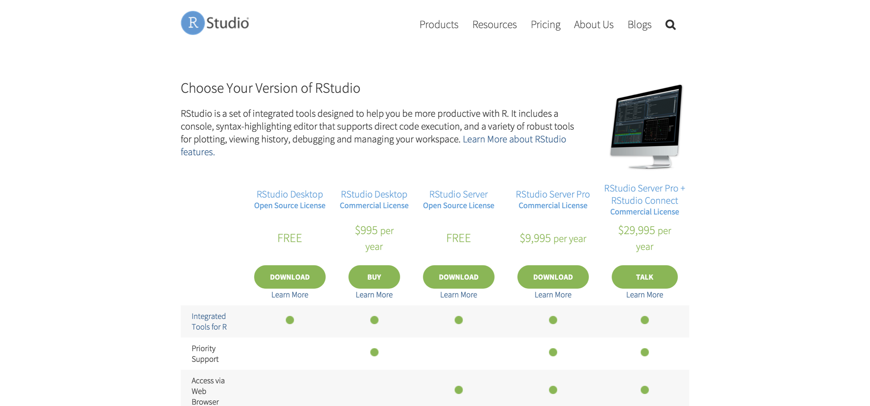 FIGURE 14.3: RStudio Downloads Page
After launching RStudio, you can use RStudio’s console panel to execute the code provided in this chapter.
FIGURE 14.3: RStudio Downloads Page
After launching RStudio, you can use RStudio’s console panel to execute the code provided in this chapter.
 FIGURE 14.4: RStudio Overview